6.2 기저함수 모형과 과최적화#
비선형 모형#
기본적인 선형회귀모형은 입력변수의 선형조합으로 이루어진다.
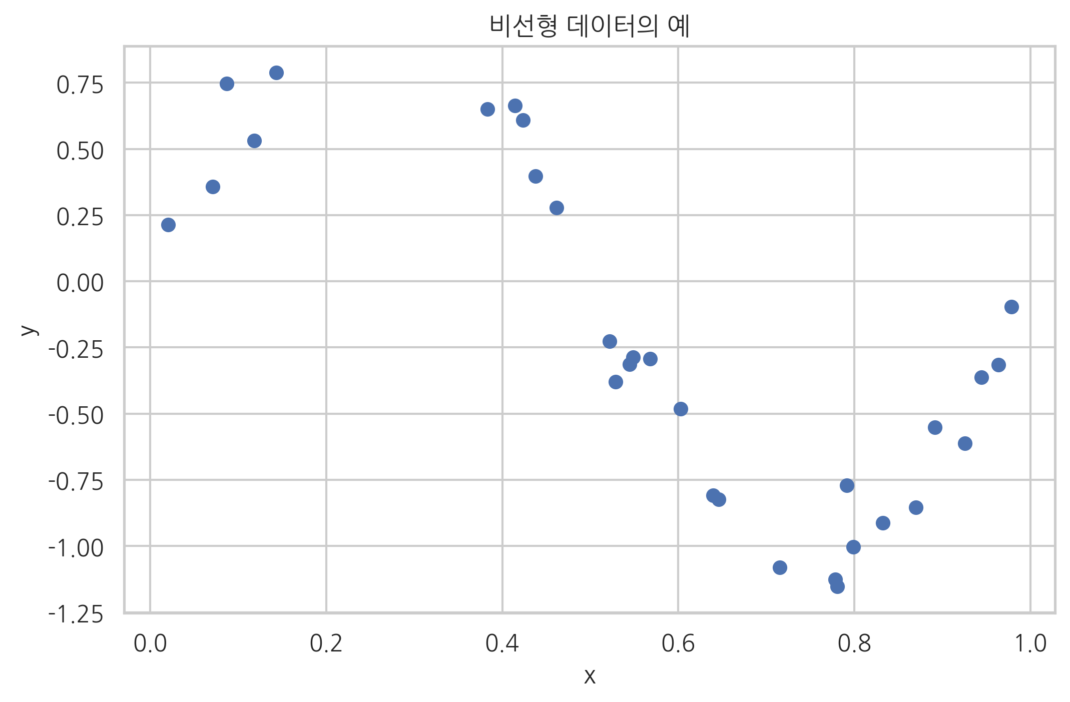
하지만 데이터가 다음 그림처럼 비선형이면 위와 같은 선형회귀모형은 적합하지 않다.
def make_nonlinear(seed=0):
    np.random.seed(seed)
    n_samples = 30
    X = np.sort(np.random.rand(n_samples))
    y = np.sin(2 * np.pi * X) + np.random.randn(n_samples) * 0.1
    X = X[:, np.newaxis]
    return (X, y)

X, y = make_nonlinear()
plt.scatter(X, y)
plt.xlabel("x")
plt.ylabel("y")
plt.title("비선형 데이터의 예")
plt.show()
이 때는 독립변수 벡터 \(x\)를 입력으로 가지는 여러개의 비선형 함수 \(\phi_j(x)\)들을 생각해 내어 원래의 입력 변수 \(x\)대신 \(\phi_j(x)\)들을 입력변수로 사용한 다음과 같은 모형을 쓰면 더 좋은 예측 성능을 가질 수도 있다.
이 새로운 모형의 모수의 갯수는 원래의 독립변수의 갯수가 아니라 우리가 생각해 낸 비선형 함수의 갯수에 의존한다.
기저함수#
하지만 이러한 비선형 모형을 만들기 위해서는 데이터에 적합한 비선형 함수를 충분히 많이 생각해 낼 수 있어야 한다. 이러한 고충을 덜기 위해 만들어진 것이 기저함수(basis function) 모형이다. 기저함수는 특정한 규칙에 따라 만들어지는 함수의 열(sequence)로서 충분히 많은 수의 함수가 있으면 어떤 모양의 함수라도 비슷하게 흉내낼 수 있는 것을 말한다.
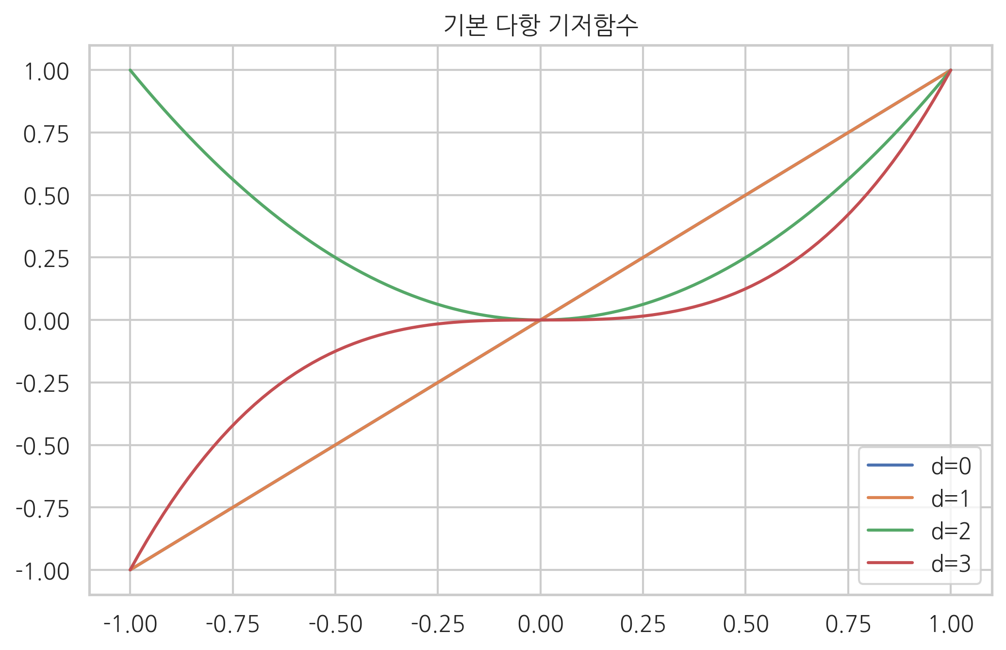
기저함수 중 가장 간단한 것이 다항 기저함수(polynomial basis function)이다.
다항회귀(polynomial regression)는 다항 기저함수를 사용하는 기저함수 모형이다. 따라서 종속 변수와 독립 변수의 관계는 다음과 같이 표현할 수 있다.
기저함수는 사람이 하나씩 생각해내는 것이 아니라 미리 만들어진 규칙에 의해 자동으로 생성되므로 비선형 함수를 만들기 위해 고민할 필요가 없다.
phi_0 = np.polynomial.Polynomial.basis(1)
phi_1 = np.polynomial.Polynomial.basis(1)
phi_2 = np.polynomial.Polynomial.basis(2)
phi_3 = np.polynomial.Polynomial.basis(3)

x = np.linspace(-1, 1, 100)

plt.plot(x, phi_0(x), label="d=0")
plt.plot(x, phi_1(x), label="d=1")
plt.plot(x, phi_2(x), label="d=2")
plt.plot(x, phi_3(x), label="d=3")
plt.legend()
plt.title("기본 다항 기저함수")
plt.show()
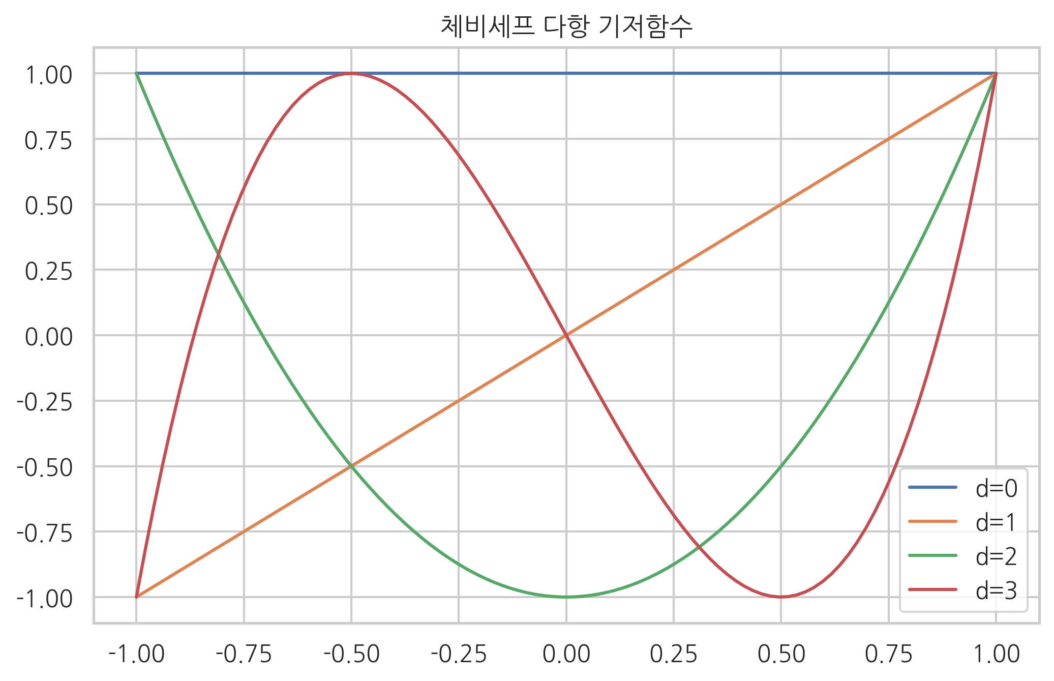
기저함수중에서도 서로 다른 두 기저함수의 곱의 정적분 값이 0이 되면 직교기저함수(orthogonal basis function)라고 한다. 체비세프 다항식은 직교기저함수의 한 예다.
phi_0 = np.polynomial.chebyshev.Chebyshev.basis(0)
phi_1 = np.polynomial.chebyshev.Chebyshev.basis(1)
phi_2 = np.polynomial.chebyshev.Chebyshev.basis(2)
phi_3 = np.polynomial.chebyshev.Chebyshev.basis(3)

x = np.linspace(-1, 1, 100)

plt.plot(x, phi_0(x), label="d=0")
plt.plot(x, phi_1(x), label="d=1")
plt.plot(x, phi_2(x), label="d=2")
plt.plot(x, phi_3(x), label="d=3")
plt.legend()
plt.title("체비세프 다항 기저함수")
plt.show()
이외에도 다음과 같은 기저함수들도 존재한다.
방사 기저함수
삼각 기저함수
시그모이드 기저함수
StatsModels를 이용한 다항회귀#
StatsModels에서는 OLS 클래스의 from_formula 메서드를 사용하여 다항회귀를 할 수 있다.
dfX = pd.DataFrame(X, columns=["x"])
dfX = sm.add_constant(dfX)
dfy = pd.DataFrame(y, columns=["y"])
df = pd.concat([dfX, dfy], axis=1)

print(sm.OLS.from_formula("y ~ x", data=df).fit().summary())
                            OLS Regression Results
==============================================================================
Dep. Variable:                      y   R-squared:                       0.565
Model:                            OLS   Adj. R-squared:                  0.549
Method:                 Least Squares   F-statistic:                     36.36
Date:                Sun, 23 Jun 2019   Prob (F-statistic):           1.69e-06
Time:                        17:40:22   Log-Likelihood:                -15.360
No. Observations:                  30   AIC:                             34.72
Df Residuals:                      28   BIC:                             37.52
Df Model:                           1
Covariance Type:            nonrobust
==============================================================================
                 coef    std err          t      P>|t|      [0.025      0.975]
------------------------------------------------------------------------------
Intercept      0.7140      0.176      4.064      0.000       0.354       1.074
x             -1.6422      0.272     -6.030      0.000      -2.200      -1.084
==============================================================================
Omnibus:                        3.728   Durbin-Watson:                   0.259
Prob(Omnibus):                  0.155   Jarque-Bera (JB):                1.766
Skew:                           0.257   Prob(JB):                        0.414
Kurtosis:                       1.928   Cond. No.                         4.85
==============================================================================

Warnings:
[1] Standard Errors assume that the covariance matrix of the errors is correctly specified.
print(sm.OLS.from_formula("y ~ x + I(x**2)", data=df).fit().summary())
                            OLS Regression Results
==============================================================================
Dep. Variable:                      y   R-squared:                       0.577
Model:                            OLS   Adj. R-squared:                  0.545
Method:                 Least Squares   F-statistic:                     18.38
Date:                Sun, 23 Jun 2019   Prob (F-statistic):           9.14e-06
Time:                        17:40:22   Log-Likelihood:                -14.953
No. Observations:                  30   AIC:                             35.91
Df Residuals:                      27   BIC:                             40.11
Df Model:                           2
Covariance Type:            nonrobust
==============================================================================
                 coef    std err          t      P>|t|      [0.025      0.975]
------------------------------------------------------------------------------
Intercept      0.8638      0.248      3.487      0.002       0.356       1.372
x             -2.4942      1.025     -2.432      0.022      -4.598      -0.390
I(x ** 2)      0.8295      0.962      0.862      0.396      -1.145       2.804
==============================================================================
Omnibus:                        3.235   Durbin-Watson:                   0.280
Prob(Omnibus):                  0.198   Jarque-Bera (JB):                1.622
Skew:                           0.235   Prob(JB):                        0.445
Kurtosis:                       1.962   Cond. No.                         23.0
==============================================================================

Warnings:
[1] Standard Errors assume that the covariance matrix of the errors is correctly specified.
print(sm.OLS.from_formula("y ~ x + I(x**2) + I(x**3)", data=df).fit().summary())
                            OLS Regression Results
==============================================================================
Dep. Variable:                      y   R-squared:                       0.956
Model:                            OLS   Adj. R-squared:                  0.951
Method:                 Least Squares   F-statistic:                     186.7
Date:                Sun, 23 Jun 2019   Prob (F-statistic):           1.06e-17
Time:                        17:40:22   Log-Likelihood:                 18.883
No. Observations:                  30   AIC:                            -29.77
Df Residuals:                      26   BIC:                            -24.16
Df Model:                           3
Covariance Type:            nonrobust
==============================================================================
                 coef    std err          t      P>|t|      [0.025      0.975]
------------------------------------------------------------------------------
Intercept     -0.2039      0.109     -1.876      0.072      -0.427       0.020
x             12.2209      1.044     11.709      0.000      10.075      14.366
I(x ** 2)    -35.4061      2.452    -14.439      0.000     -40.446     -30.366
I(x ** 3)     23.5598      1.581     14.903      0.000      20.310      26.809
==============================================================================
Omnibus:                        0.801   Durbin-Watson:                   1.769
Prob(Omnibus):                  0.670   Jarque-Bera (JB):                0.816
Skew:                           0.212   Prob(JB):                        0.665
Kurtosis:                       2.313   Cond. No.                         160.
==============================================================================

Warnings:
[1] Standard Errors assume that the covariance matrix of the errors is correctly specified.
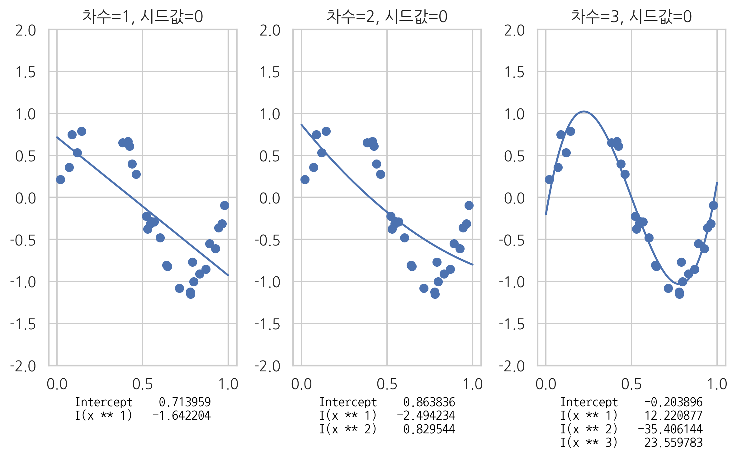
회귀분석 결과를 그림으로 그리면 다음과 같다.
def polyreg(degree, seed=0, ax=None):
    X, y = make_nonlinear(seed)

    dfX = pd.DataFrame(X, columns=["x"])
    dfX = sm.add_constant(dfX)
    dfy = pd.DataFrame(y, columns=["y"])
    df = pd.concat([dfX, dfy], axis=1)

    model_str = "y ~ "
    for i in range(degree):
        if i == 0:
            prefix = ""
        else:
            prefix = " + "
        model_str += prefix + "I(x**{})".format(i + 1)
    model = sm.OLS.from_formula(model_str, data=df)
    result = model.fit()

    if ax:
        ax.scatter(X, y)
        xx = np.linspace(0, 1, 1000)
        dfX_new = pd.DataFrame(xx[:, np.newaxis], columns=["x"])
        ax.plot(xx, result.predict(dfX_new))
        ax.set_ylim(-2, 2)
        ax.set_title("차수={}, 시드값={}".format(degree, seed))
        xlabel = "\n".join(str(result.params).split("\n")[:-1])
        font = {'family': 'NanumGothicCoding', 'color':  'black', 'size': 10}
        ax.set_xlabel(xlabel, fontdict=font)

    return result
ax1 = plt.subplot(131)
polyreg(1, ax=ax1)
ax2 = plt.subplot(132)
polyreg(2, ax=ax2)
ax3 = plt.subplot(133)
polyreg(3, ax=ax3)
plt.tight_layout()
plt.show()
과최적화#
모형을 특정 샘플 데이터에 대해 과도하게 최적화하는 것을 과최적화(overfitting)이라고 한다.
과최적화는
독립 변수 데이터 갯수에 비해 모형 모수의 수가 과도하게 크거나
독립 변수 데이터가 서로 독립이 아닌 경우에 발생한다.
이러한 상황에서는 같은 조건에 대해 답이 복수개 존재할 수 있기 때문이다.
과최적화가 문제가 되는 이유는 다음과 같다.
트레이닝에 사용되지 않은 새로운 독립 변수 값을 입력하면 오차가 커진다. (cross-validation 오차)
샘플이 조금만 변화해도 가중치 계수의 값이 크게 달라진다. (추정의 부정확함)
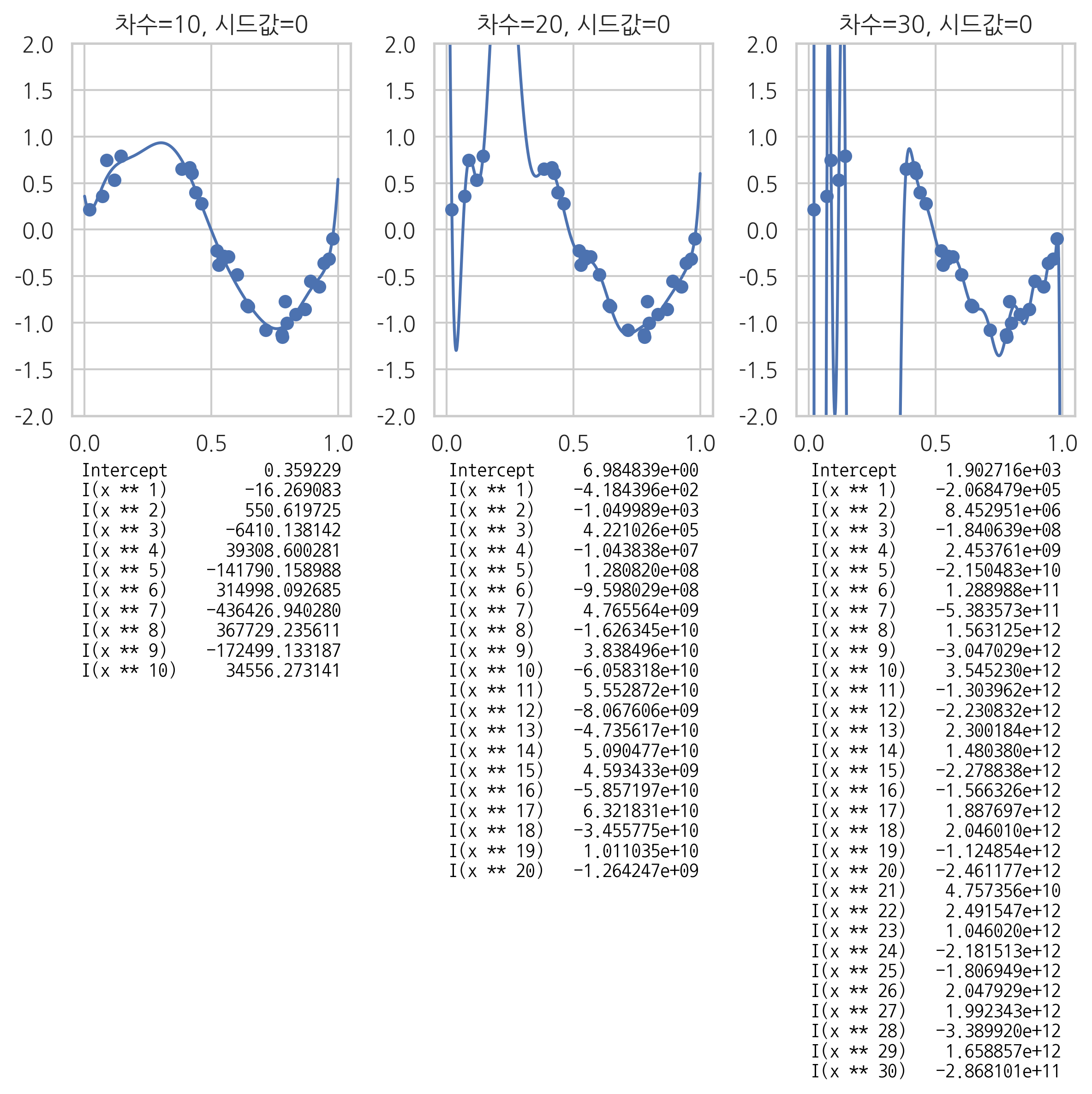
다음 그림에서 과최적화가 발생하면 주어진 데이터가 아닌 다른 새로운 x 데이터가 들어올 때 오차가 커지는 것을 볼 수 있다.
plt.figure(figsize=(8, 8))
ax1 = plt.subplot(131)
polyreg(10, ax=ax1)
ax2 = plt.subplot(132)
polyreg(20, ax=ax2)
ax3 = plt.subplot(133)
polyreg(30, ax=ax3)
plt.tight_layout()
plt.show()
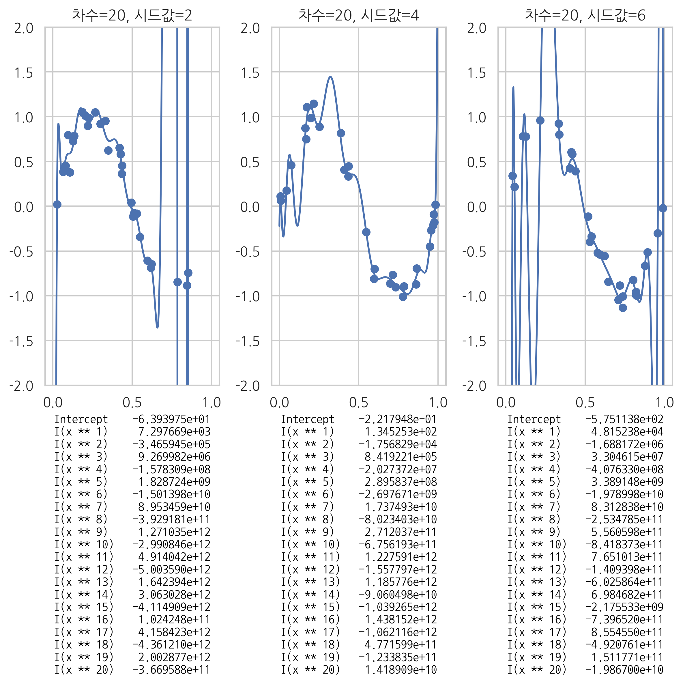
또한 데이터가 조금만 달라져도 가중치 값이 크게 달라지는 것도 확인할 수 있다.
plt.figure(figsize=(8, 8))
ax1 = plt.subplot(131)
polyreg(20, seed=2, ax=ax1)
ax2 = plt.subplot(132)
polyreg(20, seed=4, ax=ax2)
ax3 = plt.subplot(133)
polyreg(20, seed=6, ax=ax3)
plt.tight_layout()
plt.show()