비대칭 데이터 문제#
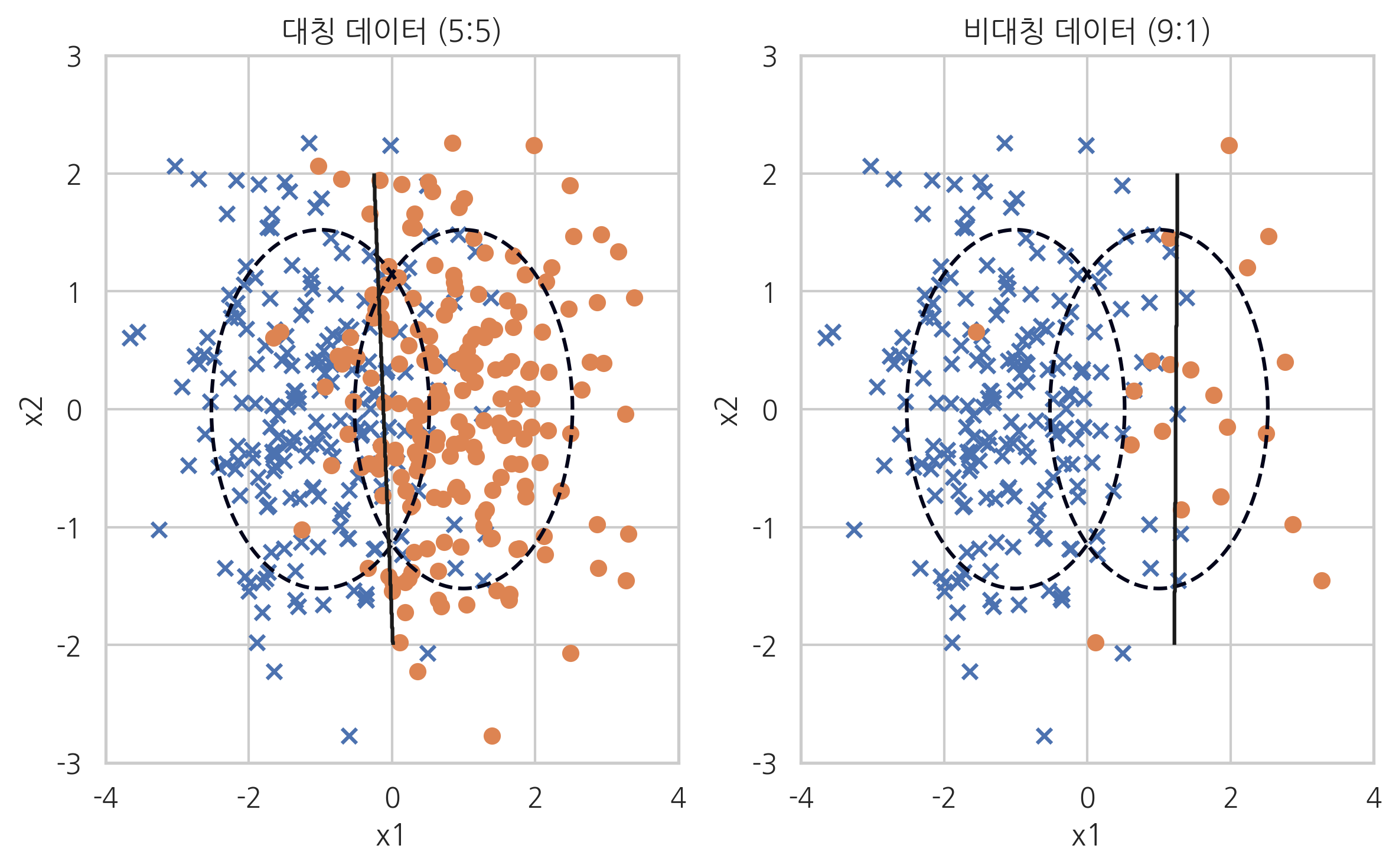
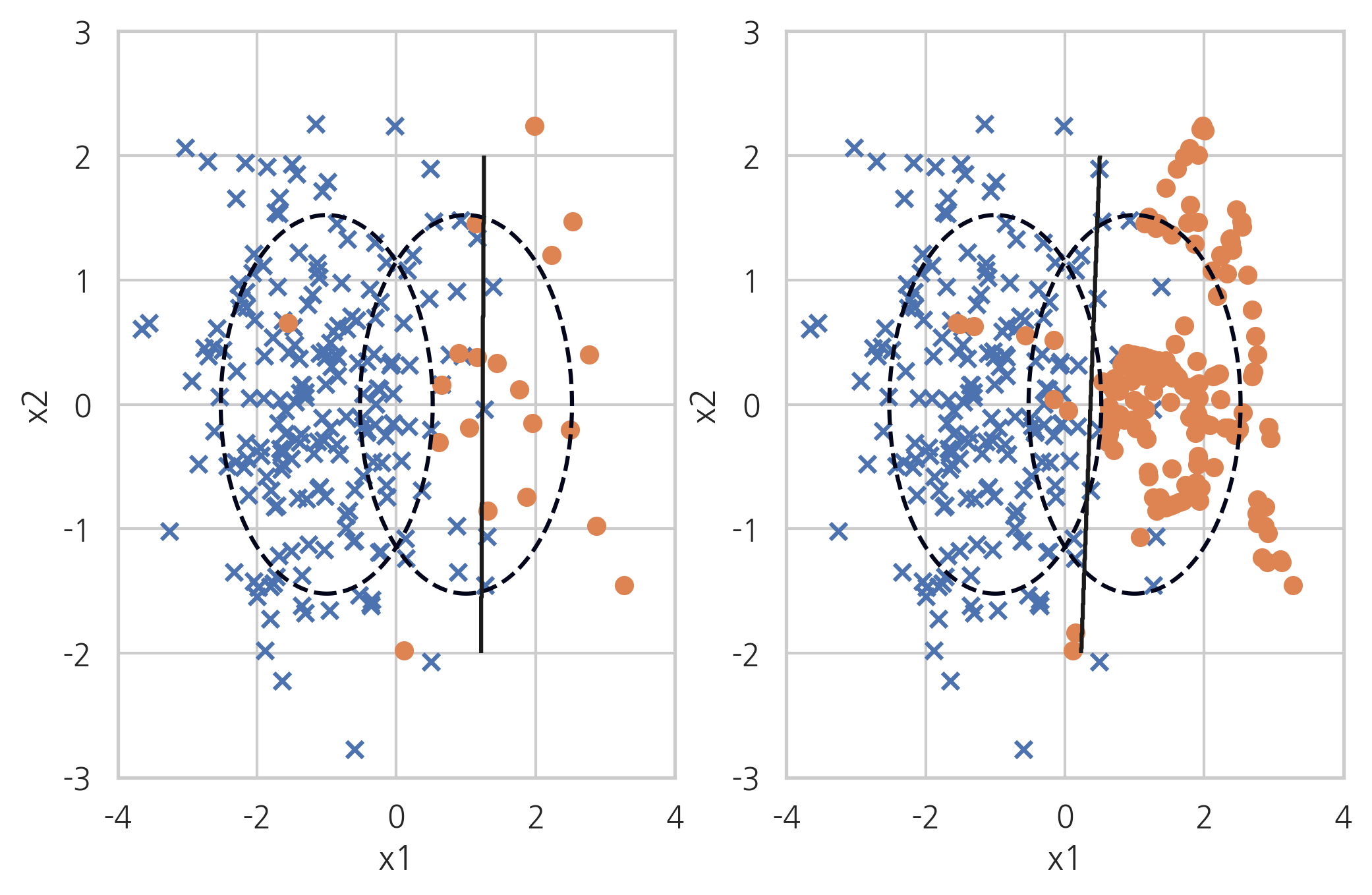
데이터 클래스 비율이 너무 차이가 나면(highly-imbalanced data) 단순히 우세한 클래스를 택하는 모형의 정확도가 높아지므로 모형의 성능판별이 어려워진다. 즉, 정확도(accuracy)가 높아도 데이터 갯수가 적은 클래스의 재현율(recall-rate)이 급격히 작아지는 현상이 발생할 수 있다.
이렇게 각 클래스에 속한 데이터의 갯수의 차이에 의해 발생하는 문제들을 비대칭 데이터 문제(imbalanced data problem)이라고 한다.
from sklearn.datasets import *
from sklearn.model_selection import train_test_split
from sklearn.metrics import recall_score
from sklearn.svm import SVC


def classification_result(n0, n1, title=""):
    rv1 = sp.stats.multivariate_normal([-1, 0], [[1, 0], [0, 1]])
    rv2 = sp.stats.multivariate_normal([+1, 0], [[1, 0], [0, 1]])
    X0 = rv1.rvs(n0, random_state=0)
    X1 = rv2.rvs(n1, random_state=0)
    X = np.vstack([X0, X1])
    y = np.hstack([np.zeros(n0), np.ones(n1)])

    x1min = -4; x1max = 4
    x2min = -2; x2max = 2
    xx1 = np.linspace(x1min, x1max, 1000)
    xx2 = np.linspace(x2min, x2max, 1000)
    X1, X2 = np.meshgrid(xx1, xx2)

    plt.contour(X1, X2, rv1.pdf(np.dstack([X1, X2])), levels=[0.05], linestyles="dashed")
    plt.contour(X1, X2, rv2.pdf(np.dstack([X1, X2])), levels=[0.05], linestyles="dashed")

    model = SVC(kernel="linear", C=1e4, random_state=0).fit(X, y)
    Y = np.reshape(model.predict(np.array([X1.ravel(), X2.ravel()]).T), X1.shape)
    plt.scatter(X[y == 0, 0], X[y == 0, 1], marker='x', label="0 클래스")
    plt.scatter(X[y == 1, 0], X[y == 1, 1], marker='o', label="1 클래스")
    plt.contour(X1, X2, Y, colors='k', levels=[0.5])
    y_pred = model.predict(X)
    plt.xlim(-4, 4)
    plt.ylim(-3, 3)
    plt.xlabel("x1")
    plt.ylabel("x2")
    plt.title(title)

    return model, X, y, y_pred

plt.subplot(121)
model1, X1, y1, y_pred1 = classification_result(200, 200, "대칭 데이터 (5:5)")
plt.subplot(122)
model2, X2, y2, y_pred2 = classification_result(200, 20, "비대칭 데이터 (9:1)")
plt.tight_layout()
plt.show()
from sklearn.metrics import classification_report, confusion_matrix

print(classification_report(y1, y_pred1))
print(classification_report(y2, y_pred2))
              precision    recall  f1-score   support

         0.0       0.86      0.83      0.84       200
         1.0       0.84      0.86      0.85       200

    accuracy                           0.85       400
   macro avg       0.85      0.85      0.85       400
weighted avg       0.85      0.85      0.85       400

              precision    recall  f1-score   support

         0.0       0.96      0.98      0.97       200
         1.0       0.75      0.60      0.67        20

    accuracy                           0.95       220
   macro avg       0.86      0.79      0.82       220
weighted avg       0.94      0.95      0.94       220
from sklearn.metrics import roc_curve, confusion_matrix
fpr1, tpr1, thresholds1 = roc_curve(y1, model1.decision_function(X1))
fpr2, tpr2, thresholds2 = roc_curve(y2, model2.decision_function(X2))
c1 = confusion_matrix(y1, y_pred1, labels=[1, 0])
c2 = confusion_matrix(y2, y_pred2, labels=[1, 0])
r1 = c1[0, 0] / (c1[0, 0] + c1[0, 1])
r2 = c2[0, 0] / (c2[0, 0] + c2[0, 1])
f1 = c1[1, 0] / (c1[1, 0] + c1[1, 1])
f2 = c2[1, 0] / (c2[1, 0] + c2[1, 1])
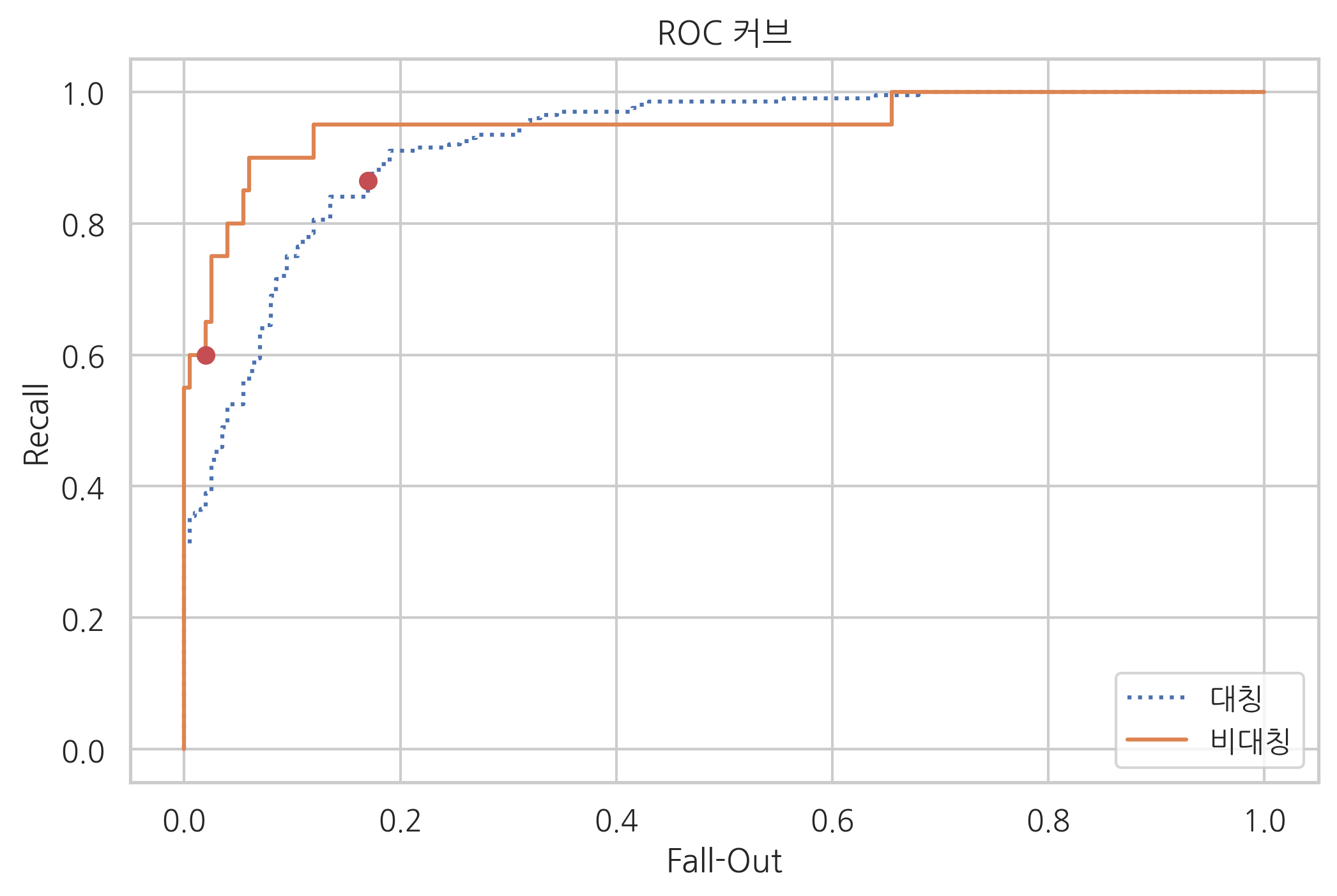
plt.plot(fpr1, tpr1, ':', label="대칭")
plt.plot(fpr2, tpr2, '-', label="비대칭")
plt.plot([f1], [r1], 'ro')
plt.plot([f2], [r2], 'ro')
plt.legend()
plt.xlabel('Fall-Out')
plt.ylabel('Recall')
plt.title('ROC 커브')
plt.show()
해결 방법#
비대칭 데이터는 다수 클래스 데이터에서 일부만 사용하는 언더 샘플링이나 소수 클래스 데이터를 증가시키는 오버 샘플링을 사용하여 데이터 비율을 맞추면 정밀도(precision)가 향상된다.
오버샘플링(Over-Sampling)
언더샘플링(Under-Sampling)
복합샘플링(Combining Over-and Under-Sampling)
imbalanced-learn 패키지#
imbalanced data 문제를 해결하기 위한 다양한 샘플링 방법을 구현한 파이썬 패키지
pip install -U imbalanced-learn
언더 샘플링#
RandomUnderSampler: random under-sampling methodTomekLinks: Tomek’s link methodCondensedNearestNeighbour: condensed nearest neighbour methodOneSidedSelection: under-sampling based on one-sided selection methodEditedNearestNeighbours: edited nearest neighbour methodNeighbourhoodCleaningRule: neighbourhood cleaning rule
from imblearn.under_sampling import *

n0 = 200; n1 = 20
rv1 = sp.stats.multivariate_normal([-1, 0], [[1, 0], [0, 1]])
rv2 = sp.stats.multivariate_normal([+1, 0], [[1, 0], [0, 1]])
X0 = rv1.rvs(n0, random_state=0)
X1 = rv2.rvs(n1, random_state=0)
X_imb = np.vstack([X0, X1])
y_imb = np.hstack([np.zeros(n0), np.ones(n1)])

x1min = -4; x1max = 4
x2min = -2; x2max = 2
xx1 = np.linspace(x1min, x1max, 1000)
xx2 = np.linspace(x2min, x2max, 1000)
X1, X2 = np.meshgrid(xx1, xx2)

def classification_result2(X, y, title=""):
    plt.contour(X1, X2, rv1.pdf(np.dstack([X1, X2])), levels=[0.05], linestyles="dashed")
    plt.contour(X1, X2, rv2.pdf(np.dstack([X1, X2])), levels=[0.05], linestyles="dashed")
    model = SVC(kernel="linear", C=1e4, random_state=0).fit(X, y)
    Y = np.reshape(model.predict(np.array([X1.ravel(), X2.ravel()]).T), X1.shape)
    plt.scatter(X[y == 0, 0], X[y == 0, 1], marker='x', label="0 클래스")
    plt.scatter(X[y == 1, 0], X[y == 1, 1], marker='o', label="1 클래스")
    plt.contour(X1, X2, Y, colors='k', levels=[0.5])
    y_pred = model.predict(X)
    plt.xlim(-4, 4)
    plt.ylim(-3, 3)
    plt.xlabel("x1")
    plt.ylabel("x2")
    plt.title(title)
    return model
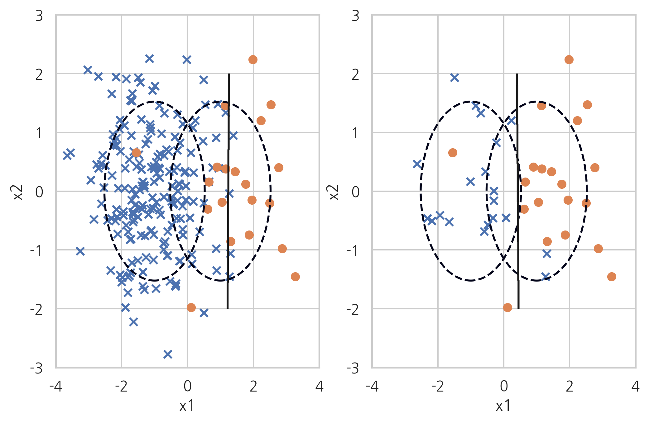
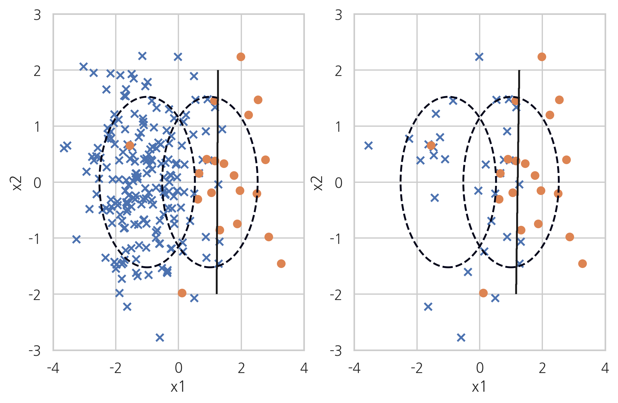
Ramdom Under-Sampler#
무작위로 데이터를 없애는 단순 샘플링
X_samp, y_samp = RandomUnderSampler(random_state=0).fit_sample(X_imb, y_imb)

plt.subplot(121)
classification_result2(X_imb, y_imb)
plt.subplot(122)
model_samp = classification_result2(X_samp, y_samp)
print(classification_report(y_imb, model_samp.predict(X_imb)))
              precision    recall  f1-score   support

         0.0       0.99      0.92      0.95       200
         1.0       0.51      0.90      0.65        20

    accuracy                           0.91       220
   macro avg       0.75      0.91      0.80       220
weighted avg       0.95      0.91      0.92       220
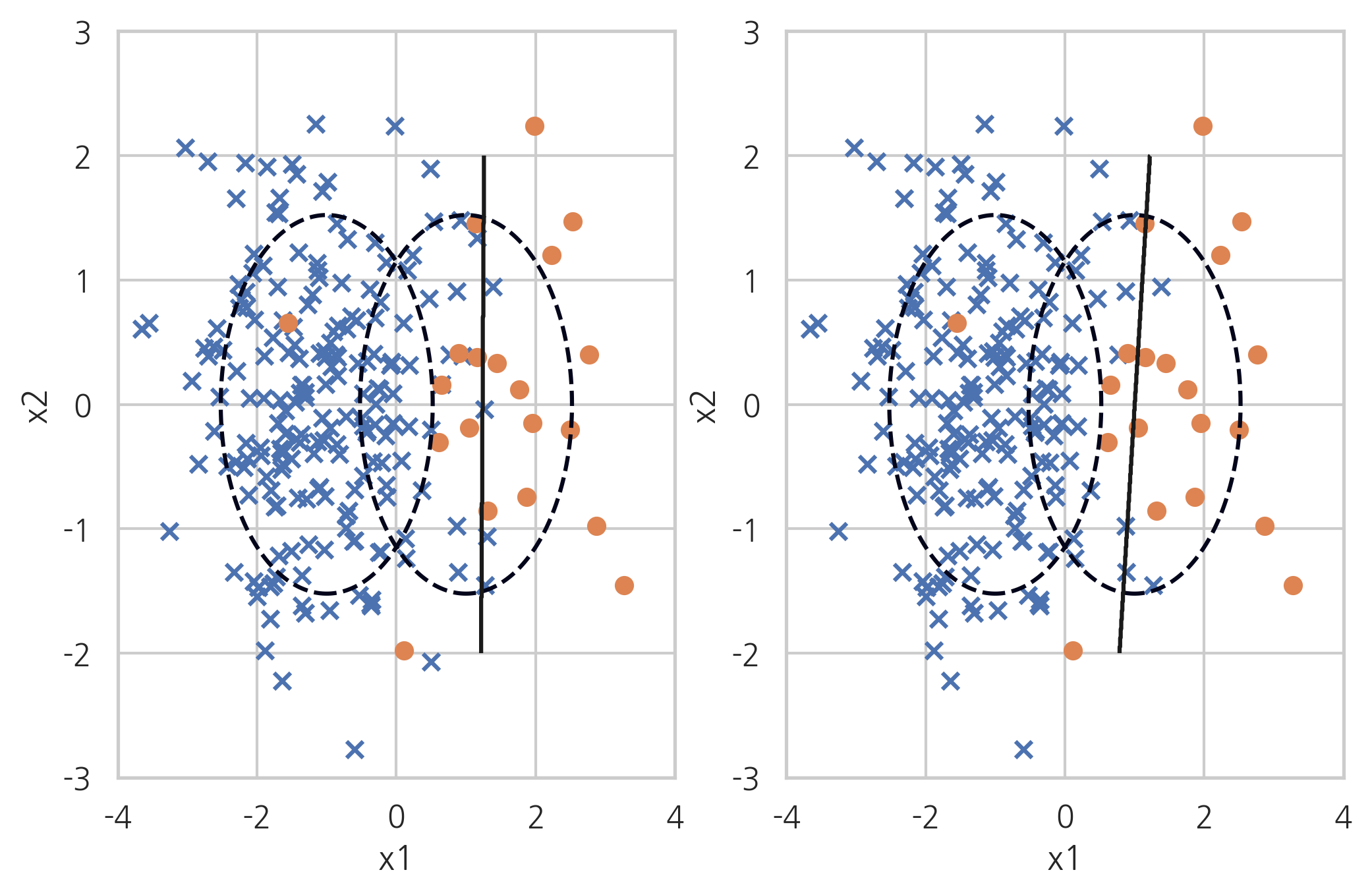
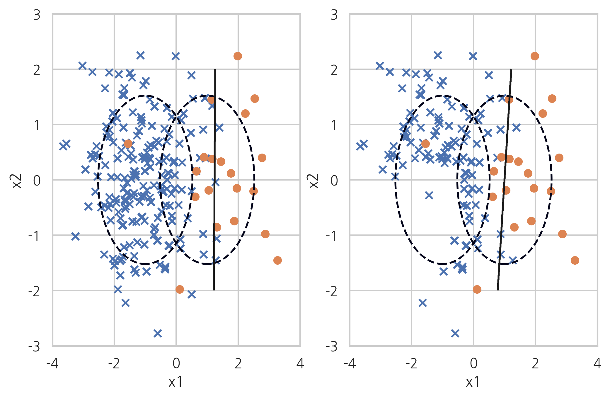
Tomek’s link method#
토멕링크(Tomek’s link)란 서로 다른 클래스에 속하는 한 쌍의 데이터 \((x_{+}, x_{-})\)로 서로에게 더 가까운 다른 데이터가 존재하지 않는 것이다. 즉 클래스가 다른 두 데이터가 아주 가까이 붙어있으면 토멕링크가 된다. 토멕링크 방법은 이러한 토멕링크를 찾은 다음 그 중에서 다수 클래스에 속하는 데이터를 제외하는 방법으로 경계선을 다수 클래스쪽으로 밀어붙이는 효과가 있다.

X_samp, y_samp = TomekLinks(random_state=0).fit_sample(X_imb, y_imb)

plt.subplot(121)
classification_result2(X_imb, y_imb)
plt.subplot(122)
model_samp = classification_result2(X_samp, y_samp)
print(classification_report(y_imb, model_samp.predict(X_imb)))
              precision    recall  f1-score   support

         0.0       0.97      0.97      0.97       200
         1.0       0.70      0.70      0.70        20

    accuracy                           0.95       220
   macro avg       0.83      0.83      0.83       220
weighted avg       0.95      0.95      0.95       220
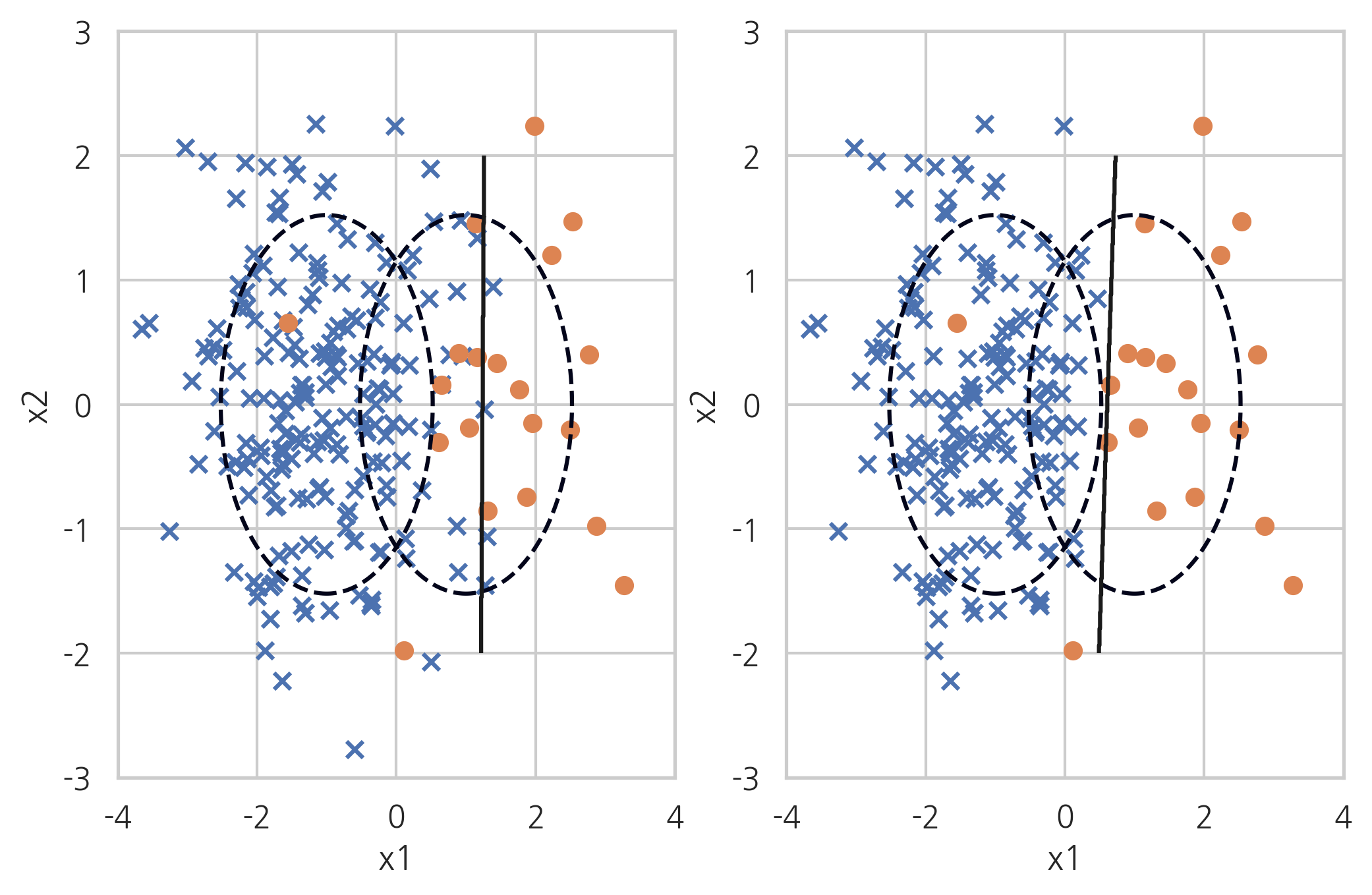
Condensed Nearest Neighbour#
CNN(Condensed Nearest Neighbour) 방법은 1-NN 모형으로 분류되지 않는 데이터만 남기는 방법이다. 선텍된 데이터 집합을 \(S\)라고 하자.
소수 클래스 데이터를 모두 \(S\)에 포함시킨다.
다수 데이터 중에서 하나를 골라서 가장 가까운 데이터가 다수 클래스이면 포함시키지 않고 아니면 \(S\)에 포함시킨다.
더이상 선택되는 데이터가 없을 때까지 2를 반복한다.
이 방법을 사용하면 기존에 선택된 데이터와 가까이 있으면서 같은 클래스인 데이터는 선택되지 않기 때문에 다수 데이터의 경우 선택되는 비율이 적어진다.
X_samp, y_samp = CondensedNearestNeighbour(random_state=0).fit_sample(X_imb, y_imb)

plt.subplot(121)
classification_result2(X_imb, y_imb)
plt.subplot(122)
model_samp = classification_result2(X_samp, y_samp)
print(classification_report(y_imb, model_samp.predict(X_imb)))
              precision    recall  f1-score   support

         0.0       0.96      0.98      0.97       200
         1.0       0.75      0.60      0.67        20

    accuracy                           0.95       220
   macro avg       0.86      0.79      0.82       220
weighted avg       0.94      0.95      0.94       220
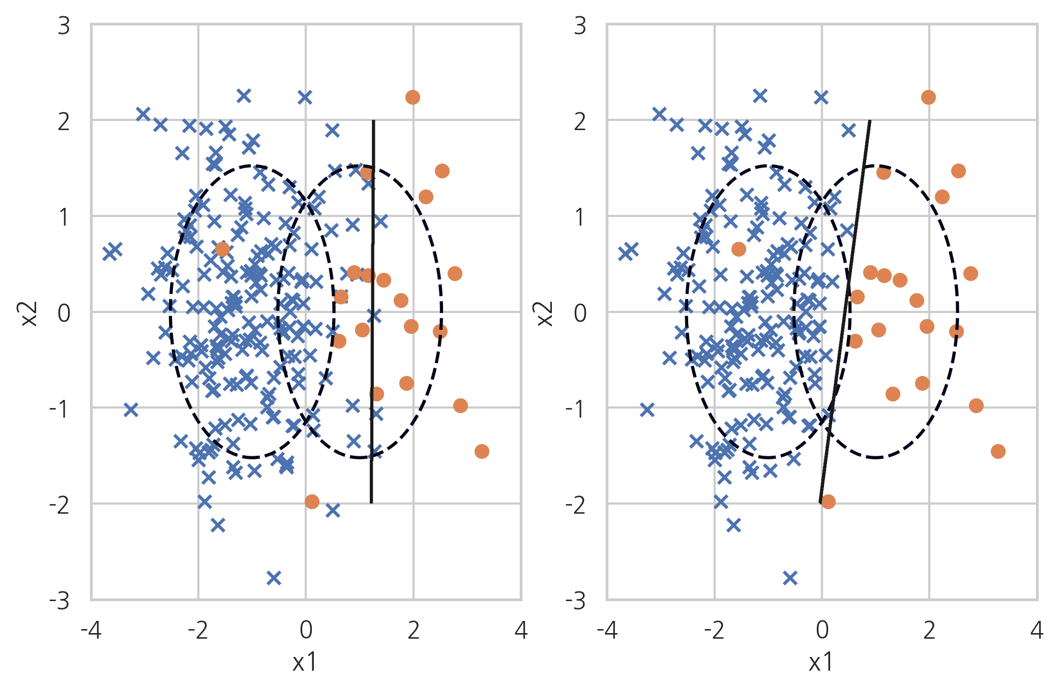
One Sided Selection#
One Sided Selection은 토맥링크 방법과 Condensed Nearest Neighbour 방법을 섞은 것이다. 토맥링크 중 다수 클래스를 제외하고 나머지 데이터 중에서도 서로 붙어있는 다수 클래스 데이터는 1-NN 방법으로 제외한다.
X_samp, y_samp = OneSidedSelection(random_state=0).fit_sample(X_imb, y_imb)

plt.subplot(121)
classification_result2(X_imb, y_imb)
plt.subplot(122)
model_samp = classification_result2(X_samp, y_samp)
print(classification_report(y_imb, model_samp.predict(X_imb)))
              precision    recall  f1-score   support

         0.0       0.97      0.97      0.97       200
         1.0       0.70      0.70      0.70        20

    accuracy                           0.95       220
   macro avg       0.83      0.83      0.83       220
weighted avg       0.95      0.95      0.95       220
Edited Nearest Neighbours#
ENN(Edited Nearest Neighbours) 방법은 다수 클래스 데이터 중 가장 가까운 k(n_neighbors)개의 데이터가 모두(kind_sel="all") 또는 다수(kind_sel="mode") 다수 클래스가 아니면 삭제하는 방법이다. 소수 클래스 주변의 다수 클래스 데이터는 사라진다.
X_samp, y_samp = EditedNearestNeighbours(kind_sel="all", n_neighbors=5, random_state=0).fit_sample(X_imb, y_imb)

plt.subplot(121)
classification_result2(X_imb, y_imb)
plt.subplot(122)
model_samp = classification_result2(X_samp, y_samp)
print(classification_report(y_imb, model_samp.predict(X_imb)))
              precision    recall  f1-score   support

         0.0       0.99      0.94      0.96       200
         1.0       0.58      0.90      0.71        20

    accuracy                           0.93       220
   macro avg       0.79      0.92      0.83       220
weighted avg       0.95      0.93      0.94       220
Neighbourhood Cleaning Rule#
Neighbourhood Cleaning Rule 방법은 CNN(Condensed Nearest Neighbour) 방법과 ENN(Edited Nearest Neighbours) 방법을 섞은 것이다.
X_samp, y_samp = NeighbourhoodCleaningRule(kind_sel="all", n_neighbors=5, random_state=0).fit_sample(X_imb, y_imb)

plt.subplot(121)
classification_result2(X_imb, y_imb)
plt.subplot(122)
model_samp = classification_result2(X_samp, y_samp)
print(classification_report(y_imb, model_samp.predict(X_imb)))
              precision    recall  f1-score   support

         0.0       0.99      0.93      0.96       200
         1.0       0.56      0.95      0.70        20

    accuracy                           0.93       220
   macro avg       0.78      0.94      0.83       220
weighted avg       0.96      0.93      0.94       220
오버 샘플링#
RandomOverSampler: random samplerADASYN: Adaptive Synthetic Sampling Approach for Imbalanced LearningSMOTE: Synthetic Minority Over-sampling Technique
from imblearn.over_sampling import *
RandomOverSampler#
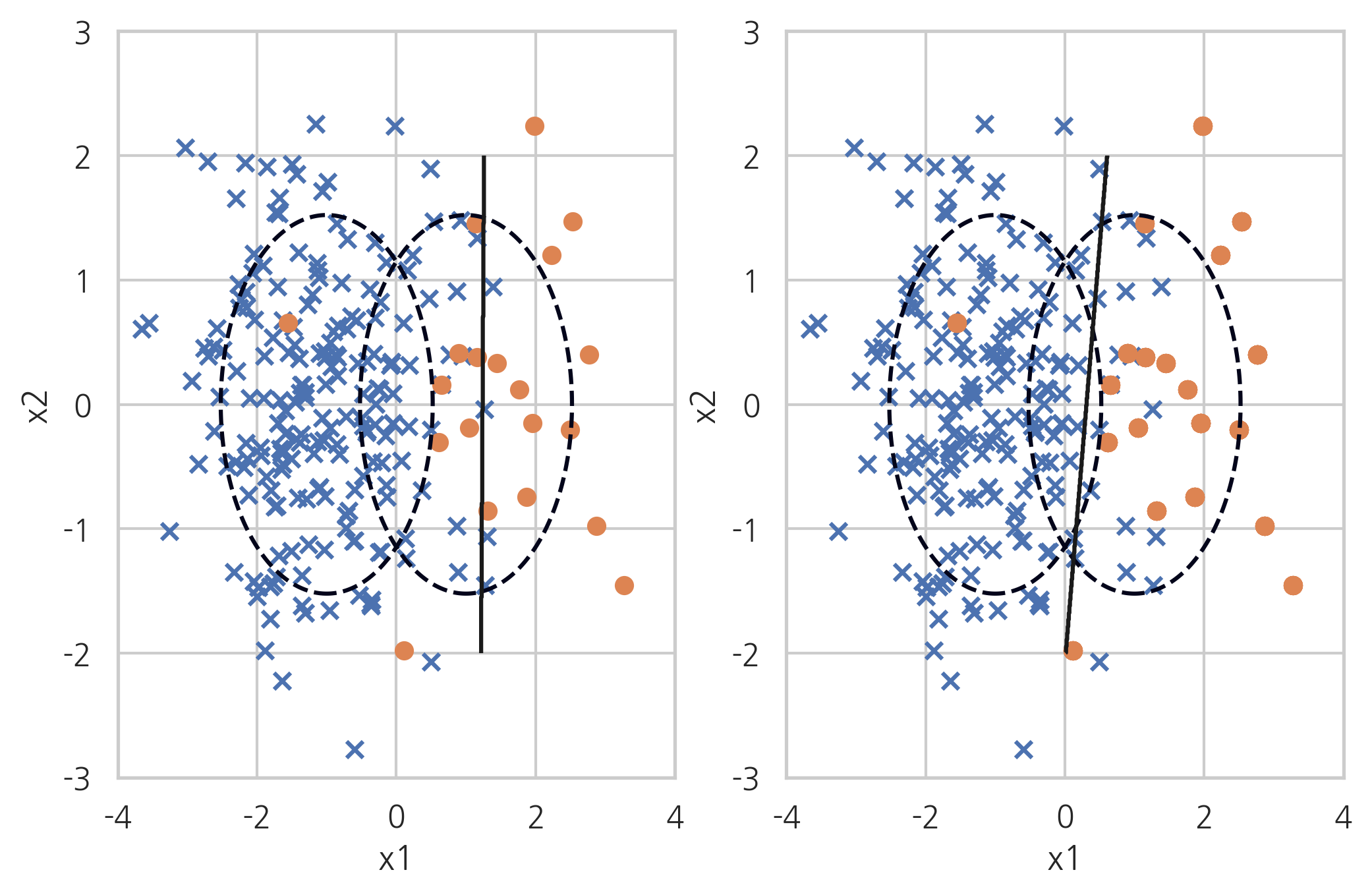
Random Over Sampling은 소수 클래스의 데이터를 반복해서 넣는 것(replacement)이다. 가중치를 증가시키는 것과 비슷하다.
X_samp, y_samp = RandomOverSampler(random_state=0).fit_sample(X_imb, y_imb)

plt.subplot(121)
classification_result2(X_imb, y_imb)
plt.subplot(122)
model_samp = classification_result2(X_samp, y_samp)
print(classification_report(y_imb, model_samp.predict(X_imb)))
              precision    recall  f1-score   support

         0.0       0.99      0.91      0.95       200
         1.0       0.51      0.95      0.67        20

    accuracy                           0.91       220
   macro avg       0.75      0.93      0.81       220
weighted avg       0.95      0.91      0.92       220
ADASYN#
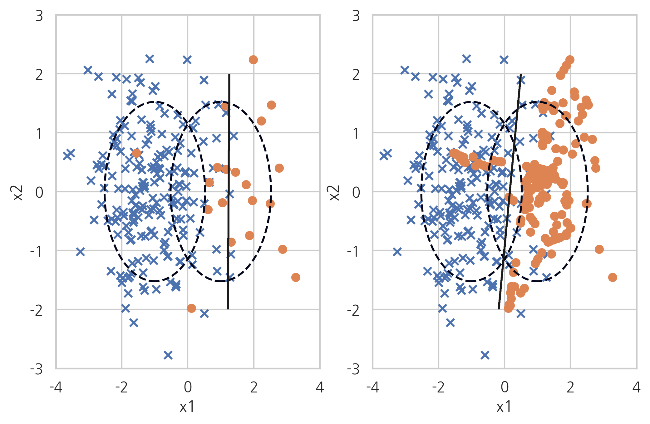
ADASYN(Adaptive Synthetic Sampling) 방법은 소수 클래스 데이터와 그 데이터에서 가장 가까운 k개의 소수 클래스 데이터 중 무작위로 선택된 데이터 사이의 직선상에 가상의 소수 클래스 데이터를 만드는 방법이다.
X_samp, y_samp = ADASYN(random_state=0).fit_sample(X_imb, y_imb)

plt.subplot(121)
classification_result2(X_imb, y_imb)
plt.subplot(122)
model_samp = classification_result2(X_samp, y_samp)
print(classification_report(y_imb, model_samp.predict(X_imb)))
              precision    recall  f1-score   support

         0.0       0.99      0.90      0.94       200
         1.0       0.47      0.95      0.63        20

    accuracy                           0.90       220
   macro avg       0.73      0.92      0.79       220
weighted avg       0.95      0.90      0.91       220
SMOTE#
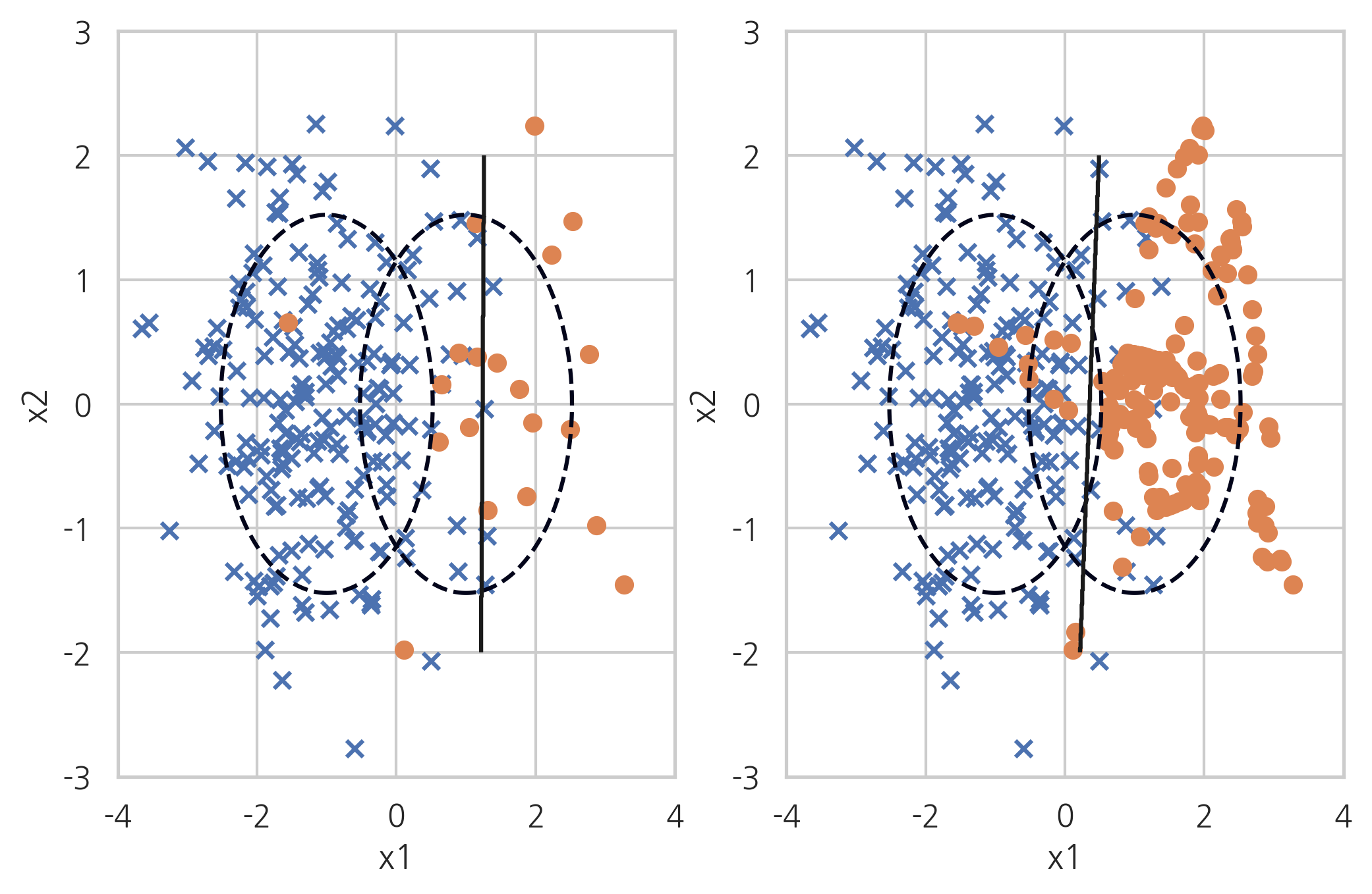
SMOTE(Synthetic Minority Over-sampling Technique) 방법도 ADASYN 방법처럼 데이터를 생성하지만 생성된 데이터를 무조건 소수 클래스라고 하지 않고 분류 모형에 따라 분류한다.

X_samp, y_samp = SMOTE(random_state=4).fit_sample(X_imb, y_imb)

plt.subplot(121)
classification_result2(X_imb, y_imb)
plt.subplot(122)
model_samp = classification_result2(X_samp, y_samp)
print(classification_report(y_imb, model_samp.predict(X_imb)))
              precision    recall  f1-score   support

         0.0       0.99      0.91      0.95       200
         1.0       0.50      0.90      0.64        20

    accuracy                           0.91       220
   macro avg       0.74      0.91      0.80       220
weighted avg       0.94      0.91      0.92       220
복합 샘플링#
SMOTEENN: SMOTE + ENNSMOTETomek: SMOTE + Tomek
from imblearn.combine import *
SMOTE+ENN#
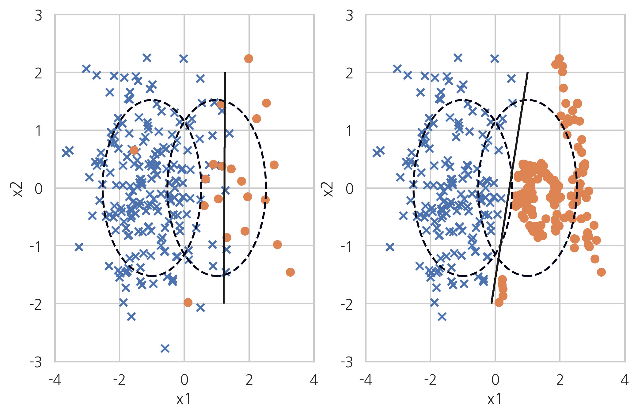
SMOTE+ENN 방법은 SMOTE(Synthetic Minority Over-sampling Technique) 방법과 ENN(Edited Nearest Neighbours) 방법을 섞은 것이다.
X_samp, y_samp = SMOTEENN(random_state=0).fit_sample(X_imb, y_imb)

plt.subplot(121)
classification_result2(X_imb, y_imb)
plt.subplot(122)
model_samp = classification_result2(X_samp, y_samp)
print(classification_report(y_imb, model_samp.predict(X_imb)))
              precision    recall  f1-score   support

         0.0       0.99      0.92      0.96       200
         1.0       0.54      0.95      0.69        20

    accuracy                           0.92       220
   macro avg       0.77      0.94      0.82       220
weighted avg       0.95      0.92      0.93       220
SMOTE+Tomek#
SMOTE+Tomek 방법은 SMOTE(Synthetic Minority Over-sampling Technique) 방법과 토멕링크 방법을 섞은 것이다.
X_samp, y_samp = SMOTETomek(random_state=4).fit_sample(X_imb, y_imb)

plt.subplot(121)
classification_result2(X_imb, y_imb)
plt.subplot(122)
model_samp = classification_result2(X_samp, y_samp)
print(classification_report(y_imb, model_samp.predict(X_imb)))
              precision    recall  f1-score   support

         0.0       0.99      0.92      0.95       200
         1.0       0.51      0.90      0.65        20

    accuracy                           0.91       220
   macro avg       0.75      0.91      0.80       220
weighted avg       0.95      0.91      0.92       220