6.4 다중공선성과 변수 선택#
다중공선성(multicollinearity)란 독립 변수의 일부가 다른 독립 변수의 조합으로 표현될 수 있는 경우이다. 독립 변수들이 서로 독립이 아니라 상호상관관계가 강한 경우에 발생한다. 이는 독립 변수의 공분산 행렬이 full rank 이어야 한다는 조건을 침해한다.
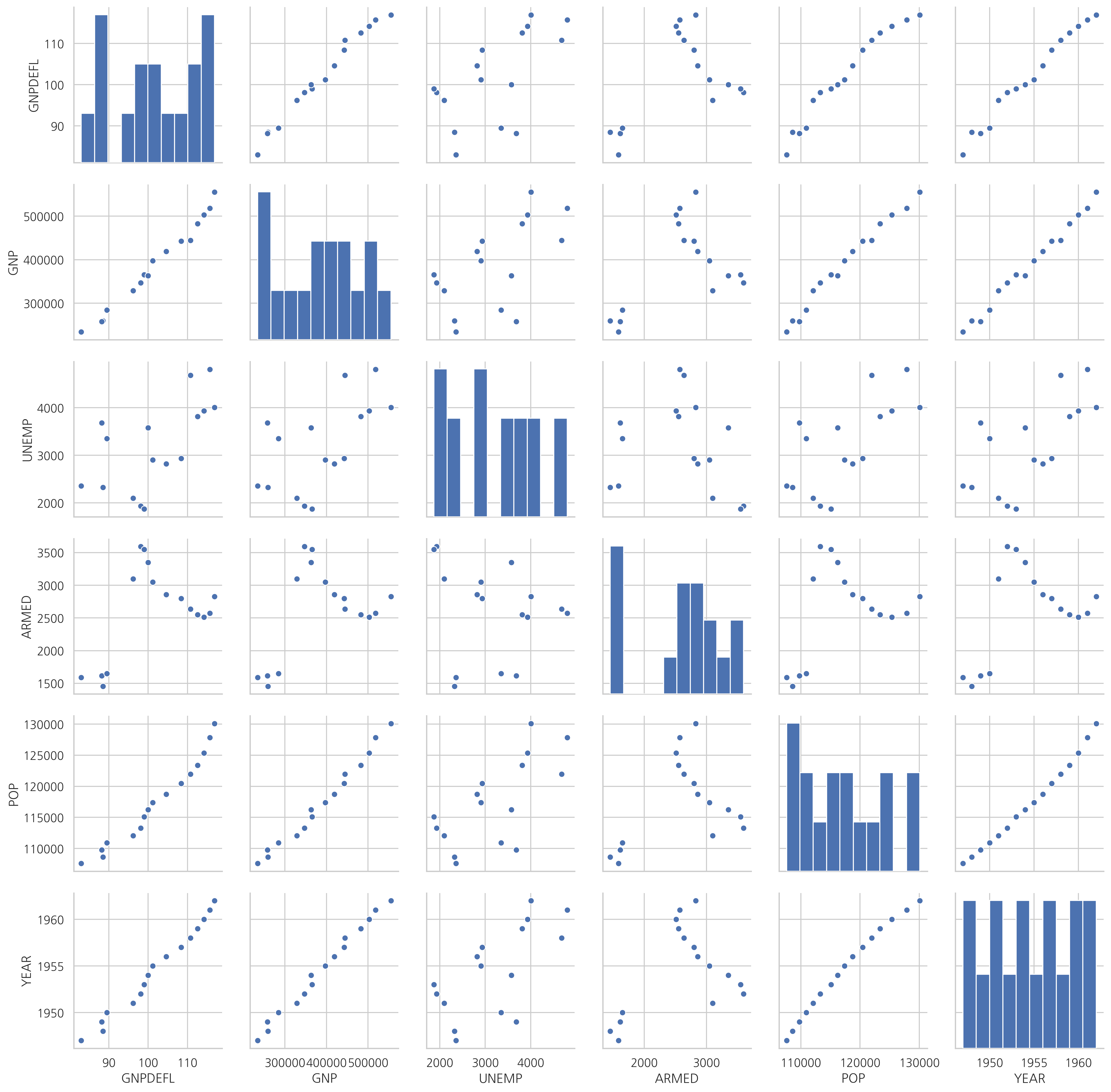
다음 데이터는 미국의 거시경제지표를 나타낸 것이다.
TOTEMP - Total Employment
GNPDEFL - GNP deflator
GNP - GNP
UNEMP - Number of unemployed
ARMED - Size of armed forces
POP - Population
YEAR - Year (1947 - 1962)
스캐터 플롯에서 보듯이 독립변수간의 상관관계가 강하다.
from statsmodels.datasets.longley import load_pandas

dfy = load_pandas().endog
dfX = load_pandas().exog
df = pd.concat([dfy, dfX], axis=1)
sns.pairplot(dfX)
plt.show()
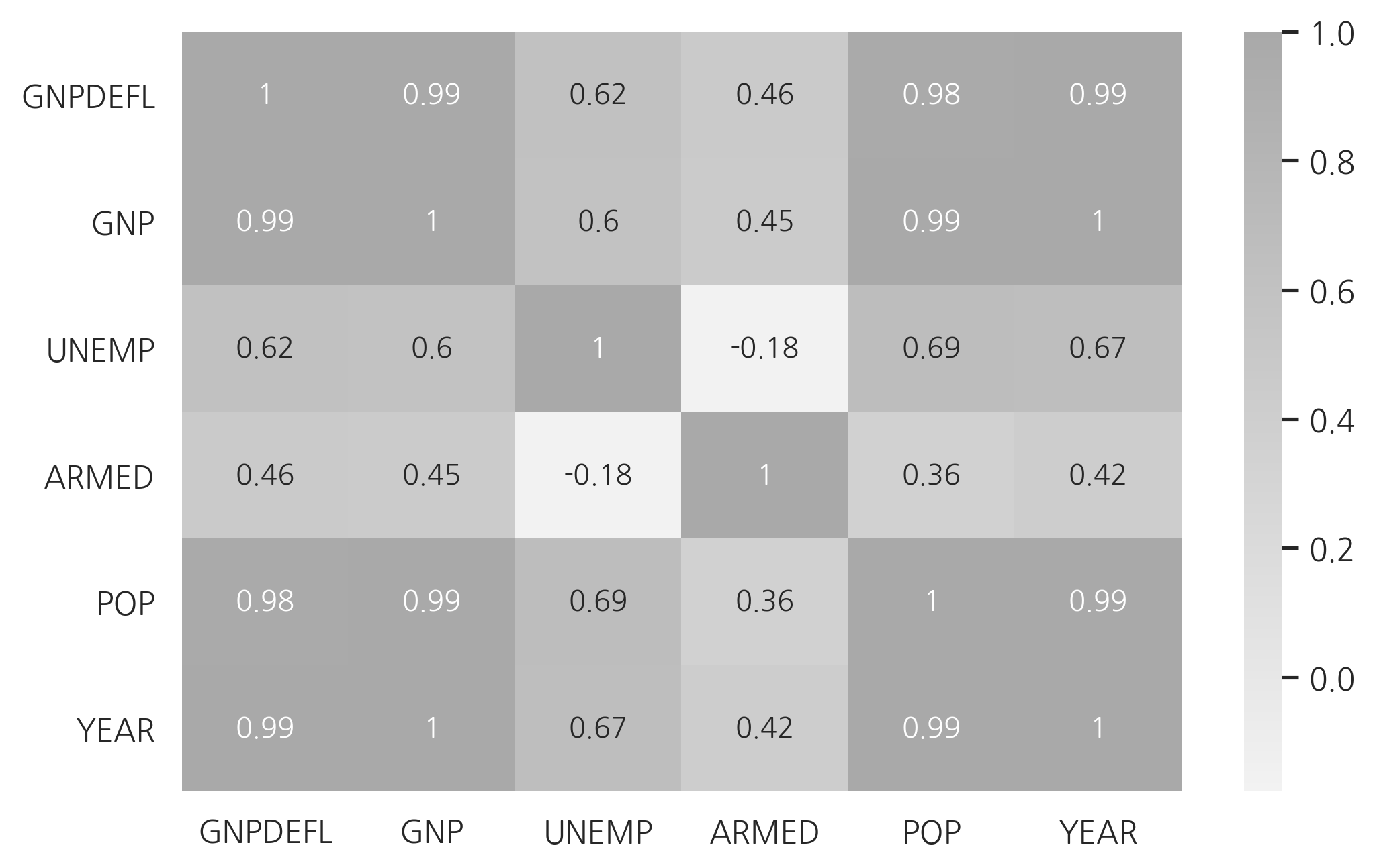
상관관계는 상관계수 행렬로도 살펴볼 수 있다.
dfX.corr()
| GNPDEFL | GNP | UNEMP | ARMED | POP | YEAR | |
|---|---|---|---|---|---|---|
| GNPDEFL | 1.000000 | 0.991589 | 0.620633 | 0.464744 | 0.979163 | 0.991149 |
| GNP | 0.991589 | 1.000000 | 0.604261 | 0.446437 | 0.991090 | 0.995273 |
| UNEMP | 0.620633 | 0.604261 | 1.000000 | -0.177421 | 0.686552 | 0.668257 |
| ARMED | 0.464744 | 0.446437 | -0.177421 | 1.000000 | 0.364416 | 0.417245 |
| POP | 0.979163 | 0.991090 | 0.686552 | 0.364416 | 1.000000 | 0.993953 |
| YEAR | 0.991149 | 0.995273 | 0.668257 | 0.417245 | 0.993953 | 1.000000 |
cmap = sns.light_palette("darkgray", as_cmap=True)
sns.heatmap(dfX.corr(), annot=True, cmap=cmap)
plt.show()
다중 공선성이 있으면 독립변수의 공분산 행렬의 조건수(conditional number)가 증가한다.
from sklearn.model_selection import train_test_split

def get_model1(seed):
    df_train, df_test = train_test_split(df, test_size=0.5, random_state=seed)
    model = sm.OLS.from_formula("TOTEMP ~ GNPDEFL + POP + GNP + YEAR + ARMED + UNEMP", data=df_train)
    return df_train, df_test, model.fit()


df_train, df_test, result1 = get_model1(3)
print(result1.summary())
                            OLS Regression Results
==============================================================================
Dep. Variable:                 TOTEMP   R-squared:                       1.000
Model:                            OLS   Adj. R-squared:                  0.997
Method:                 Least Squares   F-statistic:                     437.5
Date:                Sun, 23 Jun 2019   Prob (F-statistic):             0.0366
Time:                        18:13:38   Log-Likelihood:                -44.199
No. Observations:                   8   AIC:                             102.4
Df Residuals:                       1   BIC:                             103.0
Df Model:                           6
Covariance Type:            nonrobust
==============================================================================
                 coef    std err          t      P>|t|      [0.025      0.975]
------------------------------------------------------------------------------
Intercept  -1.235e+07   2.97e+06     -4.165      0.150      -5e+07    2.53e+07
GNPDEFL      106.2620     75.709      1.404      0.394    -855.708    1068.232
POP            2.2959      0.725      3.167      0.195      -6.915      11.506
GNP           -0.3997      0.120     -3.339      0.185      -1.920       1.121
YEAR        6300.6231   1498.900      4.203      0.149   -1.27e+04    2.53e+04
ARMED         -0.2450      0.402     -0.609      0.652      -5.354       4.864
UNEMP         -6.3311      1.324     -4.782      0.131     -23.153      10.491
==============================================================================
Omnibus:                        0.258   Durbin-Watson:                   1.713
Prob(Omnibus):                  0.879   Jarque-Bera (JB):                0.304
Skew:                           0.300   Prob(JB):                        0.859
Kurtosis:                       2.258   Cond. No.                     2.01e+10
==============================================================================

Warnings:
[1] Standard Errors assume that the covariance matrix of the errors is correctly specified.
[2] The condition number is large, 2.01e+10. This might indicate that there are
strong multicollinearity or other numerical problems.
또한 다음처럼 학습용 데이터와 검증용 데이터로 나누어 회귀분석 성능을 비교하면 과최적화가 발생하였음을 알 수 있다.
def calc_r2(df_test, result):
    target = df.loc[df_test.index].TOTEMP
    predict_test = result.predict(df_test)
    RSS = ((predict_test - target)**2).sum()
    TSS = ((target - target.mean())**2).sum()
    return 1 - RSS / TSS


test1 = []
for i in range(10):
    df_train, df_test, result = get_model1(i)
    test1.append(calc_r2(df_test, result))

test1
[0.9815050656837723,
 0.9738497543069347,
 0.9879366369871746,
 0.7588861967897188,
 0.980720608930437,
 0.8937889315168234,
 0.8798563810651999,
 0.9314665778963799,
 0.8608525682180641,
 0.9677198735170137]
독립변수가 서로 의존하게 되면 이렇게 과최적화(over-fitting) 문제가 발생하여 회귀 결과의 안정성을 해칠 가능성이 높아진다. 이를 방지하는 방법들은 다음과 같다.
변수 선택법으로 의존적인 변수 삭제
PCA(principal component analysis) 방법으로 의존적인 성분 삭제
정규화(regularized) 방법 사용
VIF#
다중 공선성을 없애는 가장 기본적인 방법은 다른 독립변수에 의존하는 변수를 없애는 것이다. 가장 의존적인 독립변수를 선택하는 방법으로는 VIF(Variance Inflation Factor)를 사용할 수 있다. VIF는 독립변수를 다른 독립변수로 선형회귀한 성능을 나타낸 것이다. \(i\)번째 변수의 VIF는 다음과 같이 계산한다.
여기에서 \(R^2_i\)는 다른 변수로 \(i\)번째 변수를 선형회귀한 성능(결정 계수)이다. 다른 변수에 의존적일 수록 VIF가 커진다.
StatsModels에서는 variance_inflation_factor 명령으로 VIF를 계산한다.
from statsmodels.stats.outliers_influence import variance_inflation_factor

vif = pd.DataFrame()
vif["VIF Factor"] = [variance_inflation_factor(
    dfX.values, i) for i in range(dfX.shape[1])]
vif["features"] = dfX.columns
vif
| VIF Factor | features | |
|---|---|---|
| 0 | 12425.514335 | GNPDEFL |
| 1 | 10290.435437 | GNP |
| 2 | 136.224354 | UNEMP |
| 3 | 39.983386 | ARMED |
| 4 | 101193.161993 | POP |
| 5 | 84709.950443 | YEAR |
상관계수와 VIF를 사용하여 독립 변수를 선택하면 GNP, ARMED, UNEMP 세가지 변수만으로도 비슷한 수준의 성능이 나온다는 것을 알 수 있다.
def get_model2(seed):
    df_train, df_test = train_test_split(df, test_size=0.5, random_state=seed)
    model = sm.OLS.from_formula("TOTEMP ~ scale(GNP) + scale(ARMED) + scale(UNEMP)", data=df_train)
    return df_train, df_test, model.fit()


df_train, df_test, result2 = get_model2(3)
print(result2.summary())
                            OLS Regression Results
==============================================================================
Dep. Variable:                 TOTEMP   R-squared:                       0.989
Model:                            OLS   Adj. R-squared:                  0.981
Method:                 Least Squares   F-statistic:                     118.6
Date:                Sun, 23 Jun 2019   Prob (F-statistic):           0.000231
Time:                        18:13:39   Log-Likelihood:                -57.695
No. Observations:                   8   AIC:                             123.4
Df Residuals:                       4   BIC:                             123.7
Df Model:                           3
Covariance Type:            nonrobust
================================================================================
                   coef    std err          t      P>|t|      [0.025      0.975]
--------------------------------------------------------------------------------
Intercept     6.538e+04    163.988    398.686      0.000    6.49e+04    6.58e+04
scale(GNP)    4338.7051    406.683     10.669      0.000    3209.571    5467.839
scale(ARMED)  -812.1407    315.538     -2.574      0.062   -1688.215      63.933
scale(UNEMP) -1373.0426    349.316     -3.931      0.017   -2342.898    -403.187
==============================================================================
Omnibus:                        0.628   Durbin-Watson:                   2.032
Prob(Omnibus):                  0.731   Jarque-Bera (JB):                0.565
Skew:                           0.390   Prob(JB):                        0.754
Kurtosis:                       1.958   Cond. No.                         4.77
==============================================================================

Warnings:
[1] Standard Errors assume that the covariance matrix of the errors is correctly specified.
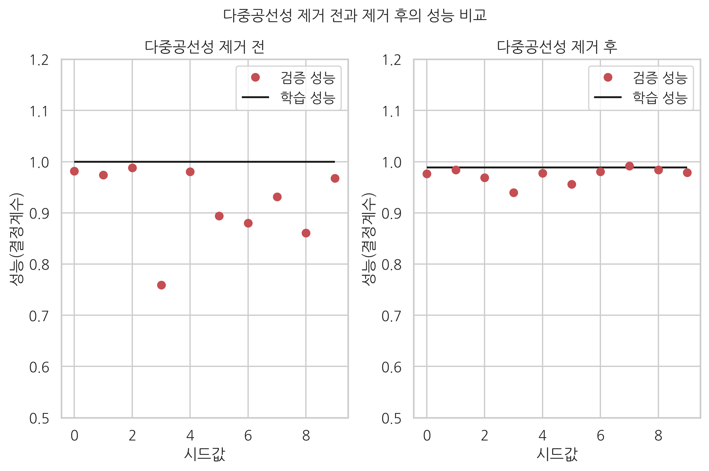
다중공선성을 제거한 경우에는 학습 성능과 검증 성능간의 차이가 줄어들었음을 확인할 수 있다. 즉, 과최적화가 발생하지 않는다.
test2 = []
for i in range(10):
    df_train, df_test, result = get_model2(i)
    test2.append(calc_r2(df_test, result))

test2
[0.9763608388904907,
 0.9841984331185702,
 0.9687069366140136,
 0.9397304053201785,
 0.9773357061188462,
 0.9561262155732316,
 0.980385249669863,
 0.9917361722470804,
 0.9837134067639467,
 0.9789512977093212]
plt.subplot(121)
plt.plot(test1, 'ro', label="검증 성능")
plt.hlines(result1.rsquared, 0, 9, label="학습 성능")
plt.legend()
plt.xlabel("시드값")
plt.ylabel("성능(결정계수)")
plt.title("다중공선성 제거 전")
plt.ylim(0.5, 1.2)

plt.subplot(122)
plt.plot(test2, 'ro', label="검증 성능")
plt.hlines(result2.rsquared, 0, 9, label="학습 성능")
plt.legend()
plt.xlabel("시드값")
plt.ylabel("성능(결정계수)")
plt.title("다중공선성 제거 후")
plt.ylim(0.5, 1.2)

plt.suptitle("다중공선성 제거 전과 제거 후의 성능 비교", y=1.04)
plt.tight_layout()
plt.show()
보스턴 집값 예측 문제에 응용#
from sklearn.datasets import load_boston
boston = load_boston()

dfX0 = pd.DataFrame(boston.data, columns=boston.feature_names)

from patsy import dmatrix

formula = "scale(CRIM) + scale(I(CRIM ** 2)) + " + \
    "scale(ZN) + scale(I(ZN ** 2)) + scale(INDUS) + " + \
    "scale(NOX) + scale(RM) + scale(AGE) + " + \
    "scale(np.log(DIS)) + scale(RAD) + scale(TAX) + " + \
    "scale(np.log(PTRATIO)) + scale(B) + scale(np.log(LSTAT)) + CHAS"
dfX = dmatrix(formula, dfX0, return_type="dataframe")
dfy = pd.DataFrame(boston.target, columns=["MEDV"])
idx_outlier = \
    np.array([7,  54, 148, 152, 160, 214, 253, 267, 364, 365, 367, 368, 369,
              371, 372, 374, 380, 385, 397, 398, 399, 400, 401, 405, 409, 410,
              412, 413, 414, 415, 416, 418, 419, 426, 445, 489, 490, 492, 505,
              161, 162, 163, 166, 186, 195, 204, 225, 257, 267, 283, 368, 369,
              370, 371, 372])

idx = list(set(range(len(dfX))).difference(idx_outlier))
dfX = dfX.iloc[idx, :].reset_index(drop=True)
dfy = dfy.iloc[idx, :].reset_index(drop=True)
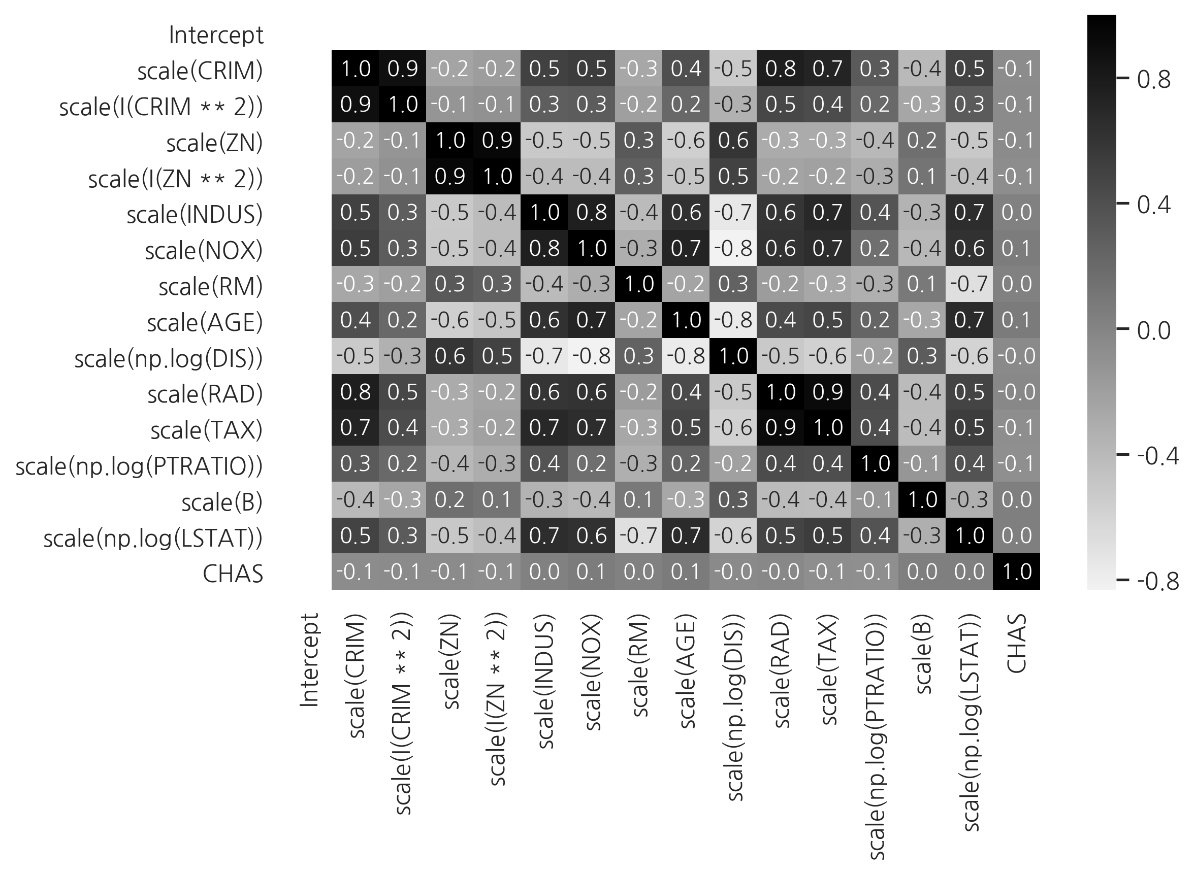
cmap = sns.light_palette("black", as_cmap=True)
sns.heatmap(dfX.corr(), annot=True, fmt='3.1f', cmap=cmap)
plt.show()
vif = pd.DataFrame()
vif["VIF Factor"] = [variance_inflation_factor(
    dfX.values, i) for i in range(dfX.shape[1])]
vif["features"] = dfX.columns
vif = vif.sort_values("VIF Factor").reset_index(drop=True)
vif
| VIF Factor | features | |
|---|---|---|
| 0 | 1.061624 | CHAS |
| 1 | 1.338325 | scale(B) |
| 2 | 1.478553 | Intercept |
| 3 | 1.780320 | scale(np.log(PTRATIO)) |
| 4 | 2.596496 | scale(RM) |
| 5 | 3.748931 | scale(AGE) |
| 6 | 3.807459 | scale(INDUS) |
| 7 | 4.682812 | scale(np.log(LSTAT)) |
| 8 | 5.071802 | scale(NOX) |
| 9 | 5.215025 | scale(np.log(DIS)) |
| 10 | 9.107858 | scale(TAX) |
| 11 | 10.218588 | scale(I(CRIM ** 2)) |
| 12 | 11.254736 | scale(RAD) |
| 13 | 11.751869 | scale(I(ZN ** 2)) |
| 14 | 14.646056 | scale(ZN) |
| 15 | 21.260182 | scale(CRIM) |
model_boston1 = sm.OLS(np.log(dfy), dfX)
result_boston1 = model_boston1.fit()
print(result_boston1.summary())
                            OLS Regression Results
==============================================================================
Dep. Variable:                   MEDV   R-squared:                       0.872
Model:                            OLS   Adj. R-squared:                  0.868
Method:                 Least Squares   F-statistic:                     199.9
Date:                Sun, 23 Jun 2019   Prob (F-statistic):          1.56e-185
Time:                        18:13:41   Log-Likelihood:                 317.45
No. Observations:                 456   AIC:                            -602.9
Df Residuals:                     440   BIC:                            -536.9
Df Model:                          15
Covariance Type:            nonrobust
==========================================================================================
                             coef    std err          t      P>|t|      [0.025      0.975]
------------------------------------------------------------------------------------------
Intercept                  3.0338      0.007    433.880      0.000       3.020       3.048
scale(CRIM)               -0.3471      0.044     -7.976      0.000      -0.433      -0.262
scale(I(CRIM ** 2))        0.3075      0.071      4.331      0.000       0.168       0.447
scale(ZN)                 -0.0465      0.022     -2.110      0.035      -0.090      -0.003
scale(I(ZN ** 2))          0.0440      0.020      2.206      0.028       0.005       0.083
scale(INDUS)               0.0037      0.012      0.323      0.747      -0.019       0.026
scale(NOX)                -0.0652      0.013     -5.001      0.000      -0.091      -0.040
scale(RM)                  0.0999      0.011      9.195      0.000       0.079       0.121
scale(AGE)                -0.0273      0.011     -2.438      0.015      -0.049      -0.005
scale(np.log(DIS))        -0.1008      0.014     -7.368      0.000      -0.128      -0.074
scale(RAD)                 0.1634      0.020      8.106      0.000       0.124       0.203
scale(TAX)                -0.0934      0.018     -5.153      0.000      -0.129      -0.058
scale(np.log(PTRATIO))    -0.0699      0.008     -8.872      0.000      -0.085      -0.054
scale(B)                   0.0492      0.007      6.699      0.000       0.035       0.064
scale(np.log(LSTAT))      -0.1487      0.013    -11.074      0.000      -0.175      -0.122
CHAS                       0.0659      0.026      2.580      0.010       0.016       0.116
==============================================================================
Omnibus:                       28.653   Durbin-Watson:                   1.309
Prob(Omnibus):                  0.000   Jarque-Bera (JB):               43.266
Skew:                           0.465   Prob(JB):                     4.03e-10
Kurtosis:                       4.188   Cond. No.                         35.2
==============================================================================

Warnings:
[1] Standard Errors assume that the covariance matrix of the errors is correctly specified.
cols = ["Intercept", "CHAS", "scale(B)", "scale(CRIM)",
        "scale(np.log(PTRATIO))", "scale(RM)", "scale(np.log(LSTAT))"]

model_boston2 = sm.OLS(np.log(dfy), dfX[cols])
result_boston2 = model_boston2.fit()
print(result_boston2.summary())
                            OLS Regression Results
==============================================================================
Dep. Variable:                   MEDV   R-squared:                       0.836
Model:                            OLS   Adj. R-squared:                  0.834
Method:                 Least Squares   F-statistic:                     380.7
Date:                Sun, 23 Jun 2019   Prob (F-statistic):          1.42e-172
Time:                        18:13:41   Log-Likelihood:                 260.52
No. Observations:                 456   AIC:                            -507.0
Df Residuals:                     449   BIC:                            -478.2
Df Model:                           6
Covariance Type:            nonrobust
==========================================================================================
                             coef    std err          t      P>|t|      [0.025      0.975]
------------------------------------------------------------------------------------------
Intercept                  3.0192      0.007    445.252      0.000       3.006       3.033
CHAS                       0.0884      0.028      3.141      0.002       0.033       0.144
scale(B)                   0.0558      0.008      6.989      0.000       0.040       0.072
scale(CRIM)               -0.1179      0.013     -9.120      0.000      -0.143      -0.092
scale(np.log(PTRATIO))    -0.0508      0.007     -6.936      0.000      -0.065      -0.036
scale(RM)                  0.1153      0.011     10.828      0.000       0.094       0.136
scale(np.log(LSTAT))      -0.1570      0.011    -14.179      0.000      -0.179      -0.135
==============================================================================
Omnibus:                       29.141   Durbin-Watson:                   1.113
Prob(Omnibus):                  0.000   Jarque-Bera (JB):               42.637
Skew:                           0.483   Prob(JB):                     5.51e-10
Kurtosis:                       4.145   Cond. No.                         5.91
==============================================================================

Warnings:
[1] Standard Errors assume that the covariance matrix of the errors is correctly specified.