커널 서포트 벡터 머신¶

XOR 문제¶

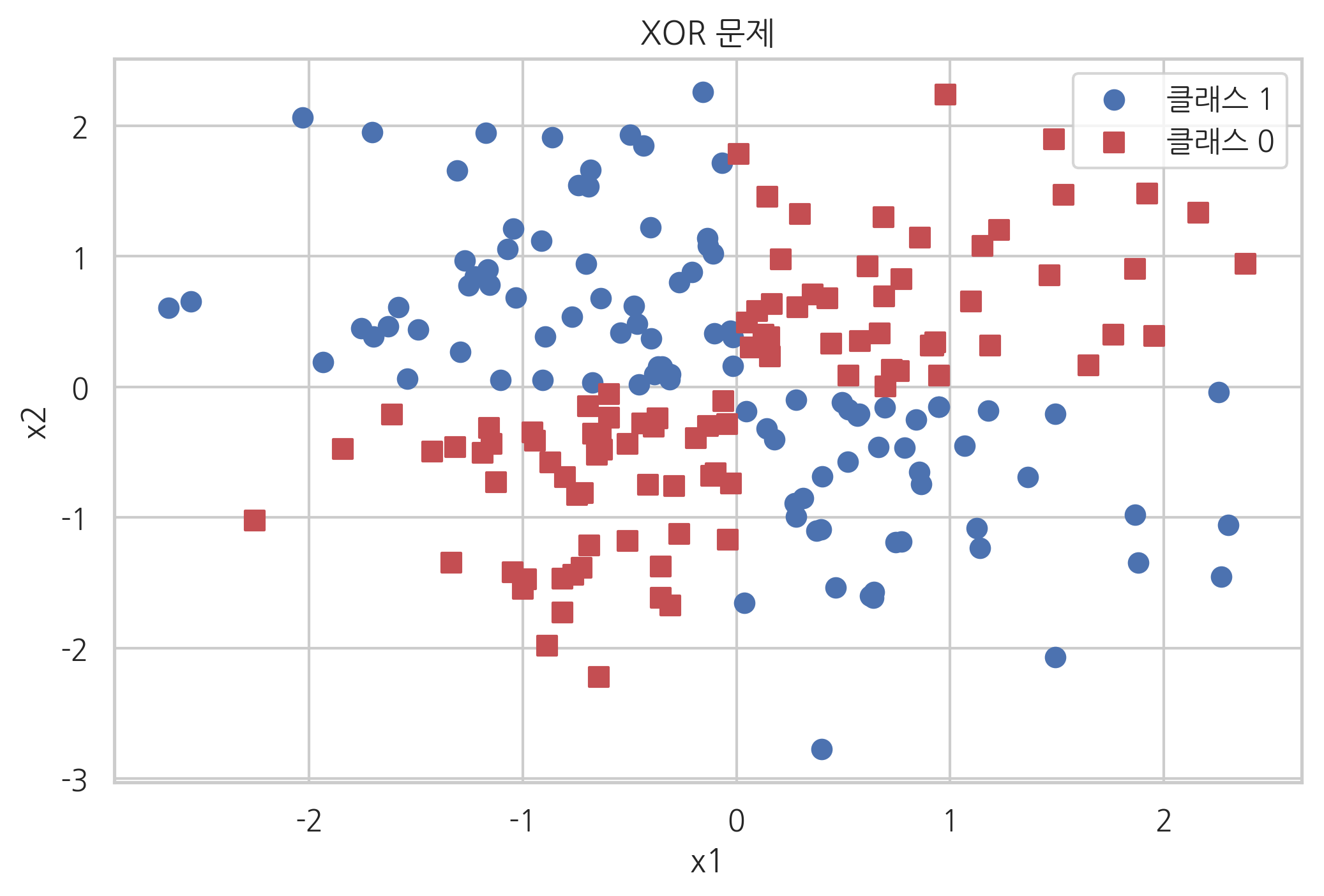
퍼셉트론이나 서포트 벡터 머신과 같은 선형판별함수 분류모형은 다음과 같은 XOR(exclusive OR) 문제를 풀지 못한다는 단점이 있다.

	X2=0	X2=1
X1=0	0	1
X1=1	1	0

이러한 경우에는 다음 그림에서 보듯이 선형판별평면(decision hyperplane)으로 영역을 나눌 수 없기 때문이다.

np.random.seed(0)
X_xor = np.random.randn(200, 2)
y_xor = np.logical_xor(X_xor[:, 0] > 0, X_xor[:, 1] > 0)
y_xor = np.where(y_xor, 1, 0)
plt.scatter(X_xor[y_xor == 1, 0], X_xor[y_xor == 1, 1],
            c='b', marker='o', label='클래스 1', s=50)
plt.scatter(X_xor[y_xor == 0, 0], X_xor[y_xor == 0, 1],
            c='r', marker='s', label='클래스 0', s=50)
plt.legend()
plt.xlabel("x1")
plt.ylabel("x2")
plt.title("XOR 문제")
plt.show()

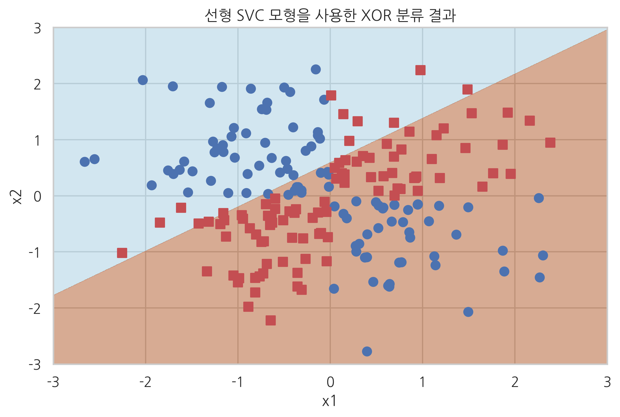
선형 SVM을 사용하면 XOR문제를 풀 수 없다.

def plot_xor(X, y, model, title, xmin=-3, xmax=3, ymin=-3, ymax=3):
    XX, YY = np.meshgrid(np.arange(xmin, xmax, (xmax-xmin)/1000),
                         np.arange(ymin, ymax, (ymax-ymin)/1000))
    ZZ = np.reshape(model.predict(
        np.array([XX.ravel(), YY.ravel()]).T), XX.shape)
    plt.contourf(XX, YY, ZZ, cmap=mpl.cm.Paired_r, alpha=0.5)
    plt.scatter(X[y == 1, 0], X[y == 1, 1], c='b',
                marker='o', label='클래스 1', s=50)
    plt.scatter(X[y == 0, 0], X[y == 0, 1], c='r',
                marker='s', label='클래스 0', s=50)
    plt.xlim(xmin, xmax)
    plt.ylim(ymin, ymax)
    plt.title(title)
    plt.xlabel("x1")
    plt.ylabel("x2")

from sklearn.svm import SVC

svc = SVC(kernel="linear").fit(X_xor, y_xor)
plot_xor(X_xor, y_xor, svc, "선형 SVC 모형을 사용한 XOR 분류 결과")
plt.show()

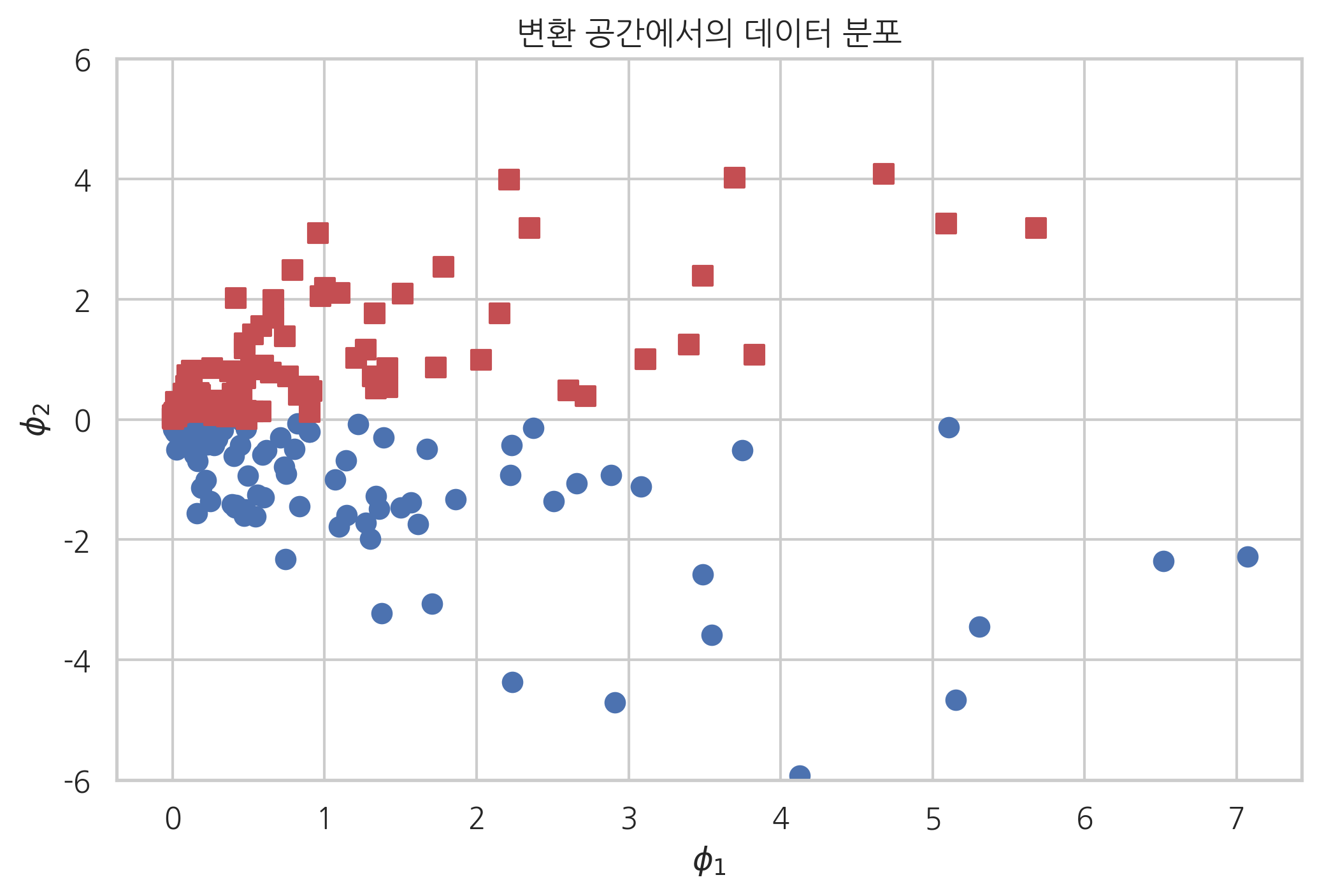
기저함수를 사용한 비선형 판별 모형¶

이러한 경우 도움이 되는 것이 원래의 $D$ 차원 독립 변수 벡터 $x$ 대신 기저함수(basis function)으로 변환한 $M$ 차원 벡터 $\phi(x)$를 독립 변수 벡터로 사용하는 방법이다.

\[ \phi(\cdot): {R}^D \rightarrow {R}^M \]

\[ x=(x_1, x_2, \cdots, x_D) \;\;\; \rightarrow \;\;\; \phi(x) = (\phi_1(x), \phi_2(x), \cdots, \phi_M(x)) \]

앞서 XOR 문제를 풀기 위해 다음과 같이 상호 곱(cross-multiplication) 항을 추가한 기저함수를 사용해 보자.

\[ (x_1, x_2) \;\;\; \rightarrow \;\;\; \phi(x) = (x_1^2, \sqrt{2}x_1x_2, x_2^2) \]

X = np.arange(6).reshape(3, 2)
X

array([[0, 1],
       [2, 3],
       [4, 5]])

FunctionTransformer 전처리 클래스로 위와 기저함수를 이용한 특징 변환을 할 수 있다.

from sklearn.preprocessing import FunctionTransformer

def basis(X):
    return np.vstack([X[:, 0]**2, np.sqrt(2)*X[:, 0]*X[:, 1], X[:, 1]**2]).T

FunctionTransformer(basis).fit_transform(X)

array([[ 0.        ,  0.        ,  1.        ],
       [ 4.        ,  8.48528137,  9.        ],
       [16.        , 28.28427125, 25.        ]])

위와 같은 기저함수를 써서 XOR 문제의 데이터를 변환하면 특성 $\phi_2$를 사용하여 클래스 분류를 할 수 있다는 것을 알 수 있다.

X_xor2 = FunctionTransformer(basis).fit_transform(X_xor)
plt.scatter(X_xor2[y_xor == 1, 0], X_xor2[y_xor == 1, 1], c="b", marker='o', s=50)
plt.scatter(X_xor2[y_xor == 0, 0], X_xor2[y_xor == 0, 1], c="r", marker='s', s=50)
plt.ylim(-6, 6)
plt.title("변환 공간에서의 데이터 분포")
plt.xlabel(r"$\phi_1$")
plt.ylabel(r"$\phi_2$")
plt.show()

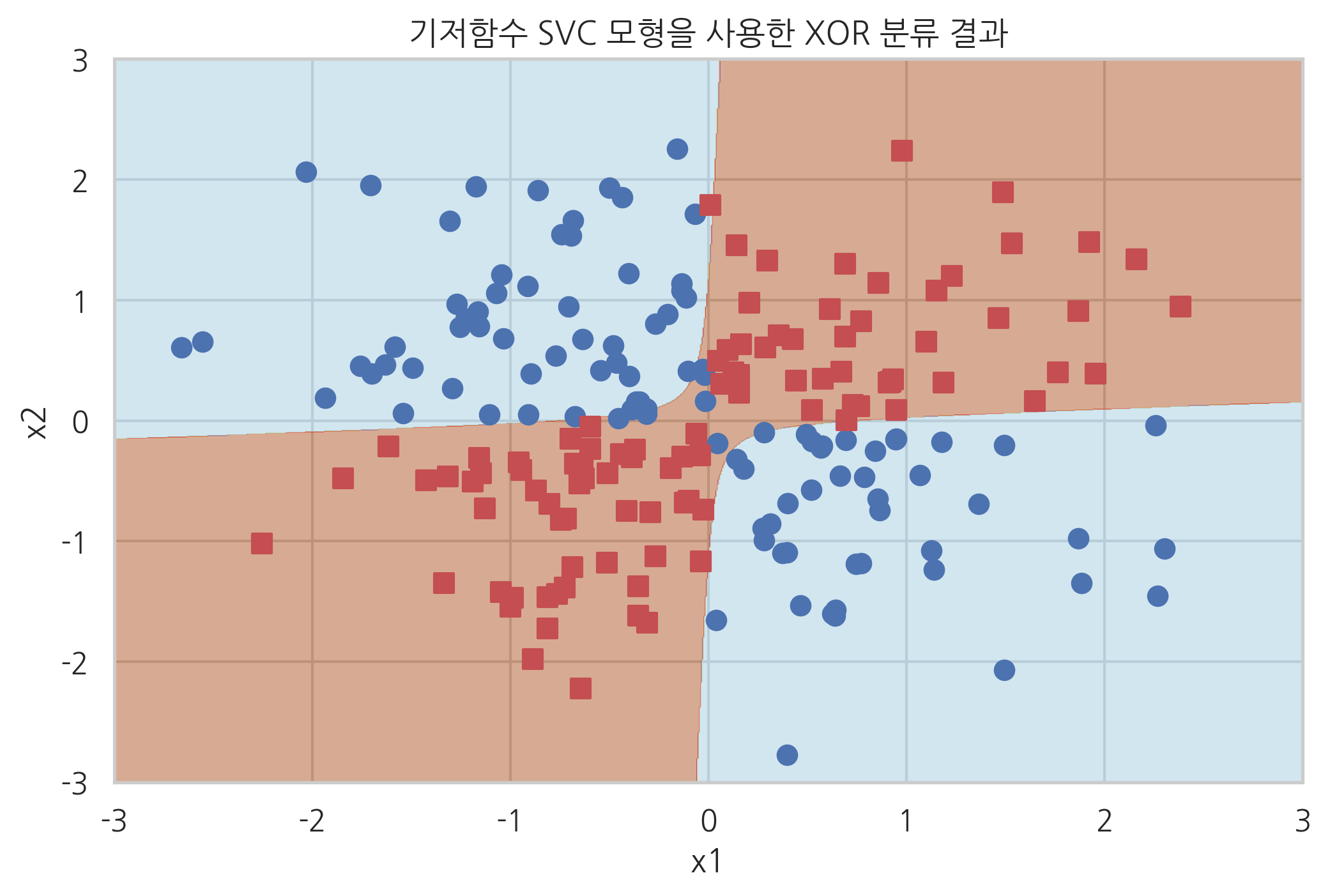
다음 코드는 Pipeline 클래스로 기저함수 전치리기와 SVC 클래스를 합친 모형의 분류 결과이다.

from sklearn.pipeline import Pipeline

basismodel = Pipeline([("basis", FunctionTransformer(basis)), 
                       ("svc", SVC(kernel="linear"))]).fit(X_xor, y_xor)
plot_xor(X_xor, y_xor, basismodel, "기저함수 SVC 모형을 사용한 XOR 분류 결과")
plt.show()

커널 트릭¶

서포트 벡터 머신의 경우 목적 함수와 예측 모형은 다음과 같은 dual form으로 표현할 수 있다.

\[ L = \sum_{n=1}^N a_n - \dfrac{1}{2}\sum_{n=1}^N\sum_{m=1}^N a_n a_m y_n y_m x_n^T x_m \]

\[ y = w^T x - w_0 = \sum_{n=1}^N a_n y_n x_n^T x - w_0 \]

이 수식에서 $x$를 기저함수 변환으로 $\phi(x)$로 바꾸면

\[ L = \sum_{n=1}^N a_n - \dfrac{1}{2}\sum_{n=1}^N\sum_{m=1}^N a_n a_m y_n y_m \phi(x_n)^T \phi(x_m) \]

\[ y = w^T x - w_0 = \sum_{n=1}^N a_n y_n \phi(x_n)^T \phi(x) - w_0 \]

이 된다. 즉 모든 기저함수는 $\phi(x_i)^T\phi(x_j)$의 형태로만 사용되며 독립적으로 사용되지 않는다.

따라서 두 개의 변환된 독립 변수 벡터를 내적(inner product) 한 값 $\phi(x_i)^T\phi(x_j)$를 하나의 함수로 나타낼 수 있다.

\[ k(x_i, x_j) = \phi(x_i)^T \phi(x_j) \]

이러한 함수를 커널(kernel)이라고 한다.

대응하는 기저함수가 존재할 수만 있다면 기저함수를 먼저 정의하고 커널을 정의하는 것이 아니라 커널을 먼저 정의해도 상관없다.

커널의 의미¶

서포트 벡터 머신의 목적 함수와 예측 모형은 커널을 사용하여 표현하면 다음과 같다.

\[ L = \sum_{n=1}^N a_n - \dfrac{1}{2}\sum_{n=1}^N\sum_{m=1}^N a_n a_m y_n y_m k(x_n, x_m) \]

\[ y = w^T x - w_0 = \sum_{n=1}^N a_n y_n k(x_n, x) - w_0 \]

커널을 사용하지 않는 경우 $ k(x, y) = x^Ty $라는 점을 고려하면 커널은 다음과 같은 특징을 보인다.

$x$와 $y$가 동일한 벡터일 때 가장 크고
두 벡터간의 거리가 멀어질 수록 작아진다.

즉, 두 표본 데이터 간의 유사도(similarity)를 측정하는 기준으로 볼 수도 있다.

커널 사용의 장점¶

커널을 사용하면 베이시스 함수를 하나씩 정의하는 수고를 덜 수 있을뿐더러 변환과 내적에 들어가는 계산량이 줄어든다. 예를 들어, 다음과 같은 기저함수의 경우

\[ \phi(x_i) = \phi([x_{i,1}, x_{i,2}]) = (x_{i,1}^2, \sqrt{2}x_{i,1}x_{i,2}, x_{i,2}^2) \]

커널 방법을 쓰지 않을 경우에 $ \phi(x_i)^T \phi(x_j) $를 계산하려면 $4 + 4 + 3 = 11$ 번의 곱셈을 해야 한다.

$\phi(x_1)$ 계산 : 곱셈 4회
$\phi(x_2)$ 계산 : 곱셈 4회
내적: 곱셈 3회

그런데 이 기저함수는 다음과 같은 커널로 대체가능하다.

\[\begin{split} \begin{eqnarray} k(x_1, x_2) &=& (x_1^Tx_2)^2 \\ &=& (x_{1,1}x_{2,1} + x_{1,2}x_{2,2})^2 \\ &=& x_{1,1}^2x_{2,1}^2 + 2x_{1,1}x_{2,1}x_{1,2}x_{2,2} + x_{1,2}^2y_{2,2}^2 \\ &=& (x_{1,1}^2, \sqrt{2}x_{1,1}x_{1,2}, x_{1,2}^2) (x_{2,1}^2, \sqrt{2}x_{2,1}x_{2,2}, x_{2,2}^2)^T \\ &=& \phi(x_1)^T \phi(x_2) \end{eqnarray} \end{split}\]

커널을 사용하면 $ \phi(x_1)^T \phi(x_2) $ 을 계산하는데 $2 + 1 = 3$ 번의 곱셈이면 된다.

$x_1^Tx_2$: 곱셈 2회
제곱: 곱셈 1회

커널의 확장 생성¶

어떤 함수가 커널함수가 된다는 것을 증명하기 위해서는 기저함수를 하나 하나 정의할 필요없이 기저함수의 내적으로 표현할 수 있다는 것만 증명하면 된다. 하지만 실제로는 다음 규칙을 이용하면 이미 만들어진 커널 $k_1(x_1, x_2)$, $k_2(x_1, x_2)$로부터 새로운 커널을 쉽게 만들 수 있다.

커널함수를 양수배한 함수는 커널함수이다. $$k(x_1, x_2) = ck_1(x_1, x_2)\;\;(c > 0)$$
커널함수에 양수인 상수를 더한 함수는 커널함수이다. $$k(x_1, x_2) = k_1(x_1, x_2) + c\;\;(c > 0)$$
두 커널함수를 더한 함수는 커널함수이다. $$k(x_1, x_2) = k_1(x_1, x_2) + k_2(x_1, x_2)$$
두 커널함수를 곱한 함수는 커널함수이다. $$k(x_1, x_2) = k_1(x_1, x_2)k_2(x_1, x_2)$$
커널함수를 $x\geq0$에서 단조증가(monotonically increasing)하는 함수에 적용하면 커널함수이다. $$k(x_1, x_2) = (k_1(x_1, x_2))^n \;\; (n=1, 2, \cdots)$$k(x_1, x_2) = \exp(k_1(x_1, x_2))$$k(x_1, x_2) = \text{sigmoid}(k_1(x_1, x_2))$$
$x_1, x_2$ 각각의 커널함수값의 곱도 커널함수이다. $$k(x_1, x_2) = k_1(x_1, x_1)k_2(x_2, x_2) $$

많이 사용되는 커널¶

다음과 같은 커널들이 많이 사용되는 커널들이다. 이 커널들은 대부분 기저함수로 변환하였을 때 무한대의 차원을 가지는 기저함수가 된다. 따라서 대부분의 비선형성을 처리할 수 있다. 비교를 위해 선형 서포트 벡터 머신의 경우도 추가하였다.

선형 서포트 벡터 머신

\[ k(x_1, x_2) = x_1^Tx_2 \]

다항 커널 (Polynomial Kernel)

\[ k(x_1, x_2) = (\gamma (x_1^Tx_2) + \theta)^d \]

RBF(Radial Basis Function) 또는 가우시안 커널(Gaussian Kernel)

\[ k(x_1, x_2) = \exp \left( -\gamma ||x_1-x_2||^2 \right) \]

시그모이드 커널 (Sigmoid Kernel)

\[ k(x_1, x_2) = \tanh(\gamma (x_1^Tx_2) + \theta) \]

앞에서 사용한 기저함수는 $\gamma = 1, \theta= 0, d=2$ 인 다항 커널임을 알 수 있다.

다항 커널¶

다항 커널은 벡터의 내적으로 정의된 커널을 확장하여 만든 커널이다. 다항 커널이 어떤 기저함수로 되어 있는지 알아보자.

간단한 경우로 $\gamma=1$, $\theta=1$, $d=3$이고 $x$가 스칼라인 경우에는

\[\begin{split} \begin{eqnarray} k(x_1, x_2) &=& (x_1^Tx_2 + 1)^4 \\ &=& x_1^4x_2^4 + 4x_1^3x_2^3 + 6x_1^2x_2^2 + 4x_1x_2 + 1 \\ &=& (x_1^4, 2x_1^3, \sqrt{6}x_1, 2x_1, 1)^T (x_2^4, 2x_2^3, \sqrt{6}x_2, 2x_2, 1) \ \\ \end{eqnarray} \end{split}\]

처럼 기저함수의 내적이 된다. 즉, 기저함수는 다음 5개가 된다.

\[\begin{split} \begin{eqnarray} \phi_1(x) &=& x^4 \\ \phi_2(x) &=& 2x^3 \\ \phi_3(x) &=& \sqrt{6}x^2 \\ \phi_4(x) &=& 2x \\ \phi_5(x) &=& 1 \\ \end{eqnarray} \end{split}\]

x1 = 1
x2 = np.linspace(-3, 3, 100)

def poly4(x1, x2):
    return (x1 * x2 + 1) ** 4

plt.figure(figsize=(8, 4))
plt.subplot(121)
plt.plot(x2, poly4(x1, x2), ls="-")
plt.xlabel("x2")
plt.title("4차 다항커널의 예")

plt.subplot(122)
plt.plot(x2, x2 ** 4)
plt.plot(x2, 2 * x2 ** 3)
plt.plot(x2, np.sqrt(6) * x2 ** 2)
plt.plot(x2, 2 * x2)
plt.plot(x2, np.ones_like(x2))
plt.xlabel("x2")
plt.title("4차 다항커널의 기저함수들")

plt.show()

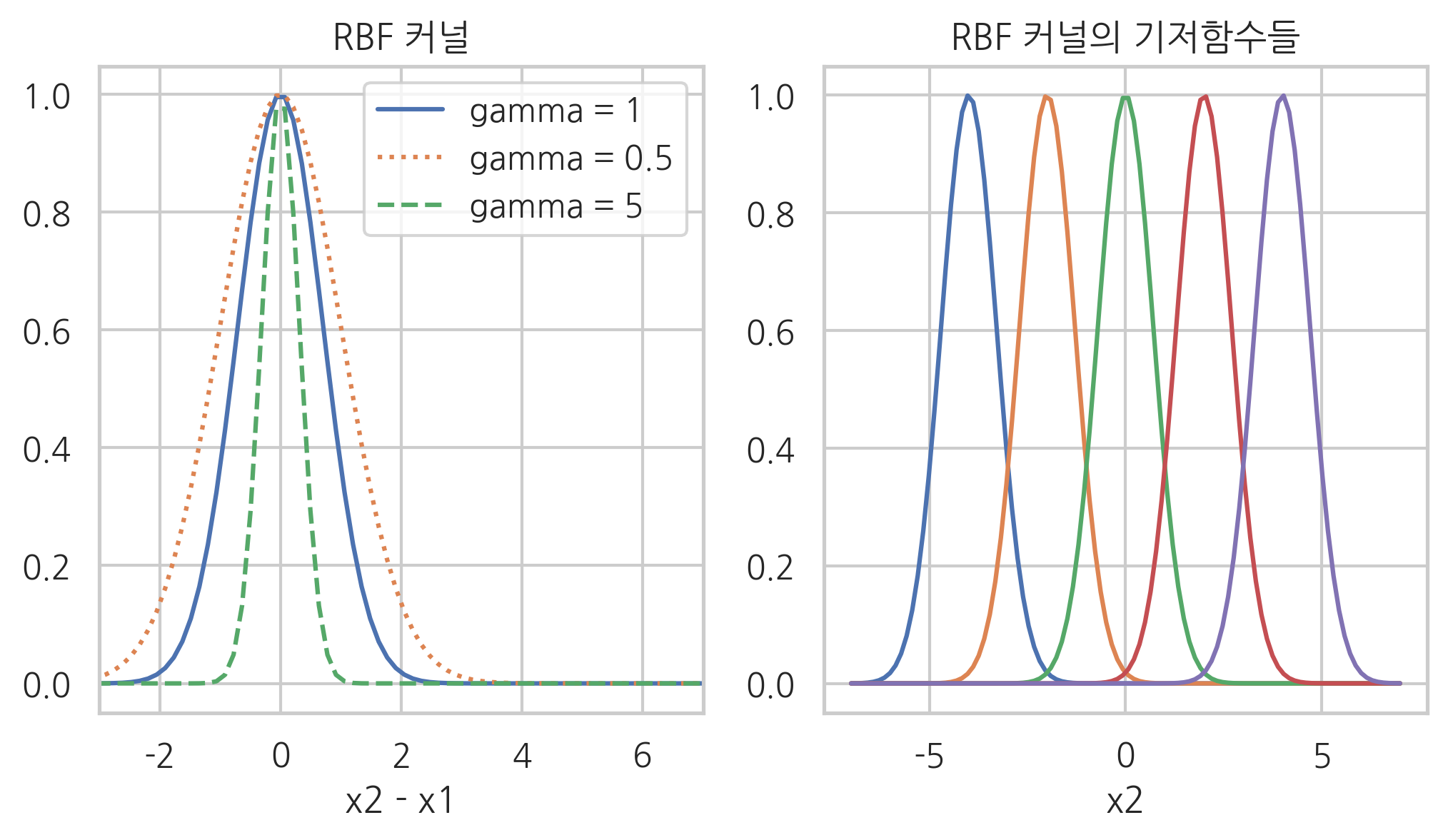
RBF 커널¶

RBF 커널은 가우시안 커널이라고도 한다. 문제를 간단하게 하기 위해 다음과 같이 가정한다.

\[ \gamma=\frac{1}{2} \]

\[ \|x_1\| = \|x_2\| = 1 \]

그러면 RBF 커널은

\[\begin{split} \begin{eqnarray} k(x_1, x_2) &=& \exp{\left(-\frac{||x_1 - x_2||^2}{2}\right)} \\ &=& \exp{\left(-\frac{x_1^Tx_1}{2} - \frac{x_2^Tx_2}{2} + 2x_1^Tx_2 \right)} \\ &=& \exp{\left(-\frac{x_1^Tx_1}{2}\right)}\exp{\left(-\frac{x_2^Tx_2}{2}\right)}\exp{(x_1^Tx_2)} \\ &=& C \exp{(x_1^Tx_2)} \\ &\approx& C \left( 1 + (x_1^Tx_2) + \dfrac{1}{2!}(x_1^Tx_2)^2 + \dfrac{1}{3!}(x_1^Tx_2)^3 + \cdots \right) \\ \end{eqnarray} \end{split}\]

에서 차수가 무한대인 다항커널과 같다.

x1 = 0.0
x2 = np.linspace(-7, 7, 100)

def rbf(x1, x2, gamma):
    return np.exp(-gamma * np.abs(x2 - x1) ** 2)

plt.figure(figsize=(8, 4))
plt.subplot(121)
plt.plot(x2, rbf(x1, x2, 1), ls="-", label="gamma = 1")
plt.plot(x2, rbf(x1, x2, 0.5), ls=":", label="gamma = 0.5")
plt.plot(x2, rbf(x1, x2, 5), ls="--", label="gamma = 5")
plt.xlabel("x2 - x1")
plt.xlim(-3, 7)
plt.legend(loc=1)
plt.title("RBF 커널")

plt.subplot(122)
plt.plot(x2, rbf(-4, x2, 1))
plt.plot(x2, rbf(-2, x2, 1))
plt.plot(x2, rbf(0, x2, 1))
plt.plot(x2, rbf(2, x2, 1))
plt.plot(x2, rbf(4, x2, 1))
plt.xlabel("x2")
plt.title("RBF 커널의 기저함수들")

plt.show()

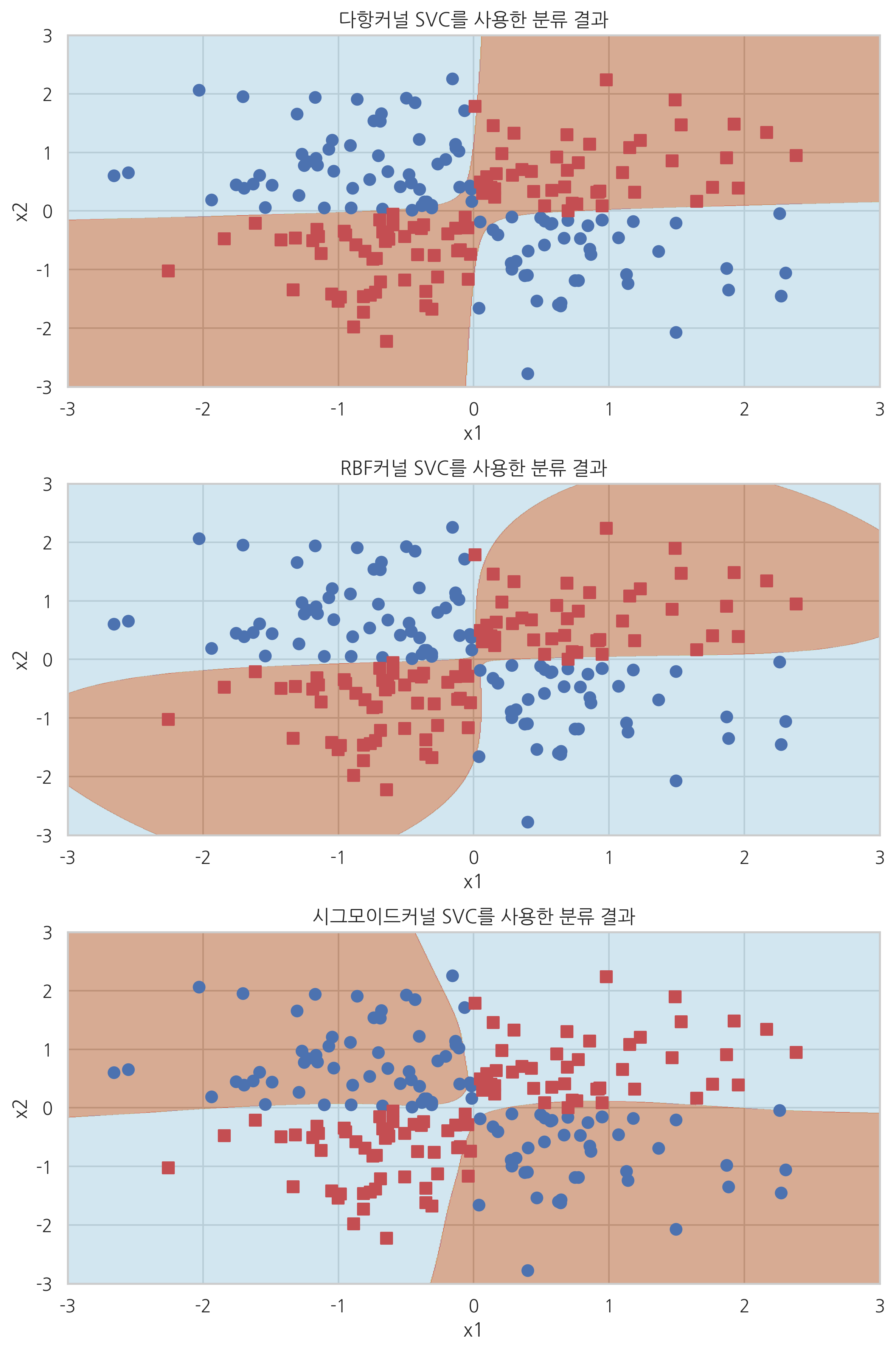
scikit-learn의 커널 SVM¶

scikit-learn의 SVM 클래스는 kernel 인수를 지정하여 커널을 설정할 수 있다.

kernel = "linear": 선형 SVM. $k(x_1, x_2) = x_1^T x_2$
kernel = "poly": 다항 커널. $k(x_1, x_2) = (\gamma (x_1^Tx_2) + \theta)^d$
- gamma: $\gamma$
- coef0: $\theta$
- degree: $d$
kernel = "rbf" 또는 kernel = None: RBF 커널. $k(x_1, x_2) = \exp \left( -\gamma ||x_1-x_2||^2 \right)$
- gamma: $\gamma$
kernel = "sigmoid": 시그모이드 커널. $k(x_1, x_2) = \tanh(\gamma (x_1^Tx_2) + \theta)$
- gamma: $\gamma$
- coef0: $\theta$

polysvc = SVC(kernel="poly", degree=2, gamma=1, coef0=0).fit(X_xor, y_xor)
rbfsvc = SVC(kernel="rbf").fit(X_xor, y_xor)
sigmoidsvc = SVC(kernel="sigmoid", gamma=2, coef0=2).fit(X_xor, y_xor)

plt.figure(figsize=(8, 12))
plt.subplot(311)
plot_xor(X_xor, y_xor, polysvc, "다항커널 SVC를 사용한 분류 결과")
plt.subplot(312)
plot_xor(X_xor, y_xor, rbfsvc, "RBF커널 SVC를 사용한 분류 결과")
plt.subplot(313)
plot_xor(X_xor, y_xor, sigmoidsvc, "시그모이드커널 SVC를 사용한 분류 결과")
plt.tight_layout()
plt.show()

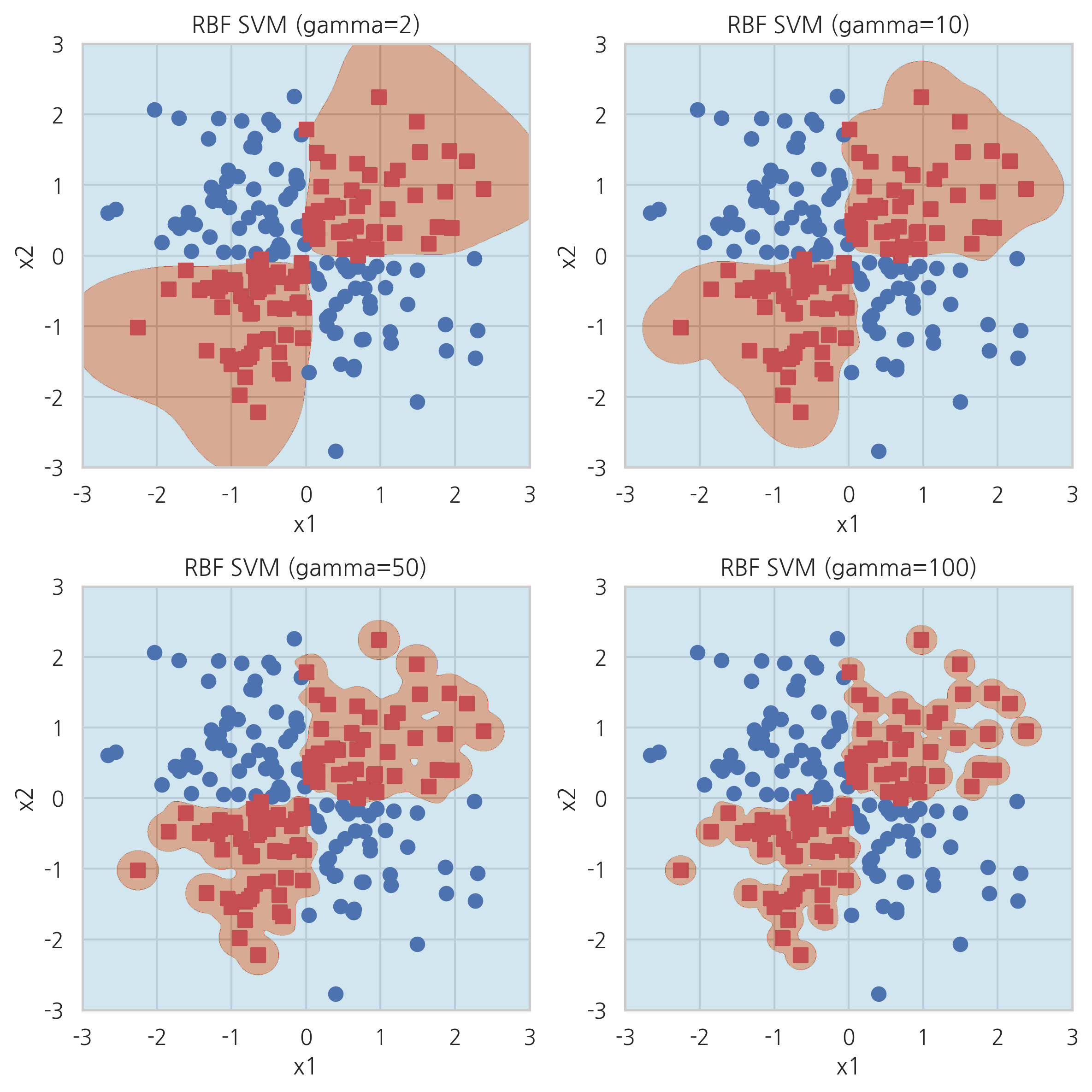
커널 파라미터의 영향¶

plt.figure(figsize=(8, 8))
plt.subplot(221)
plot_xor(X_xor, y_xor, SVC(kernel="rbf", gamma=2).fit(X_xor, y_xor), "RBF SVM (gamma=2)")
plt.subplot(222)
plot_xor(X_xor, y_xor, SVC(kernel="rbf", gamma=10).fit(X_xor, y_xor), "RBF SVM (gamma=10)")
plt.subplot(223)
plot_xor(X_xor, y_xor, SVC(kernel="rbf", gamma=50).fit(X_xor, y_xor), "RBF SVM (gamma=50)")
plt.subplot(224)
plot_xor(X_xor, y_xor, SVC(kernel="rbf", gamma=100).fit(X_xor, y_xor), "RBF SVM (gamma=100)")
plt.tight_layout()
plt.show()

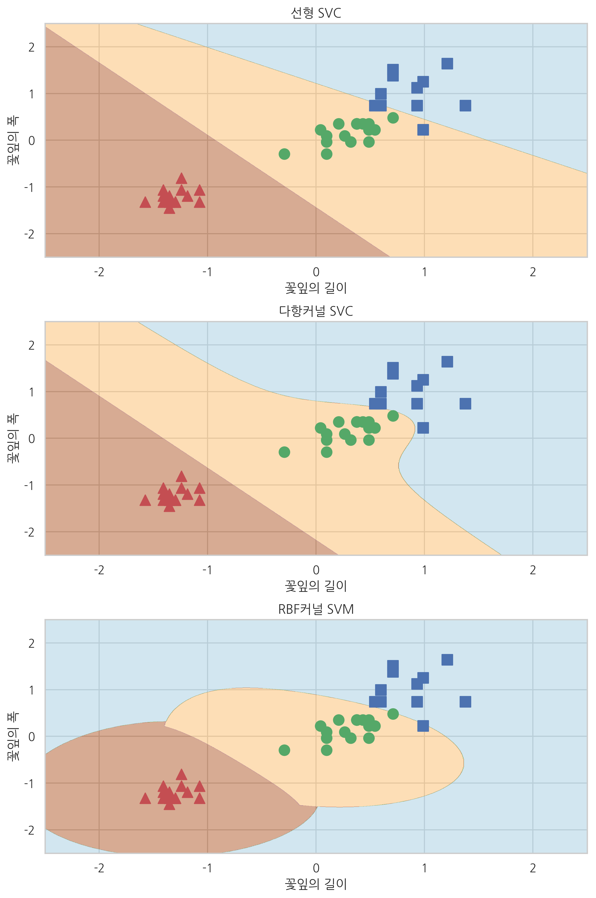
붓꽃 문제에의 응용¶

from sklearn.datasets import load_iris
from sklearn.model_selection import train_test_split
from sklearn.preprocessing import StandardScaler

iris = load_iris()
X = iris.data[:, [2, 3]]
y = iris.target
X_train, X_test, y_train, y_test = train_test_split(X, y, test_size=0.3, random_state=0)
sc = StandardScaler()
sc.fit(X_train)
X_train_std = sc.transform(X_train)
X_test_std = sc.transform(X_test)
X_combined_std = np.vstack((X_train_std, X_test_std))
y_combined = np.hstack((y_train, y_test))


def plot_iris(X, y, model, title, xmin=-2.5, xmax=2.5, ymin=-2.5, ymax=2.5):
    XX, YY = np.meshgrid(np.arange(xmin, xmax, (xmax-xmin)/1000),
                         np.arange(ymin, ymax, (ymax-ymin)/1000))
    ZZ = np.reshape(model.predict(np.array([XX.ravel(), YY.ravel()]).T), XX.shape)
    plt.contourf(XX, YY, ZZ, cmap=mpl.cm.Paired_r, alpha=0.5)
    plt.scatter(X[y == 0, 0], X[y == 0, 1], c='r', marker='^', label='0', s=100)
    plt.scatter(X[y == 1, 0], X[y == 1, 1], c='g', marker='o', label='1', s=100)
    plt.scatter(X[y == 2, 0], X[y == 2, 1], c='b', marker='s', label='2', s=100)
    plt.xlim(xmin, xmax)
    plt.ylim(ymin, ymax)
    plt.xlabel("꽃잎의 길이")
    plt.ylabel("꽃잎의 폭")
    plt.title(title)


model1 = SVC(kernel='linear').fit(X_test_std, y_test)
model2 = SVC(kernel='poly', random_state=0,
             gamma=10, C=1.0).fit(X_test_std, y_test)
model3 = SVC(kernel='rbf', random_state=0, gamma=1,
             C=1.0).fit(X_test_std, y_test)

plt.figure(figsize=(8, 12))
plt.subplot(311)
plot_iris(X_test_std, y_test, model1, "선형 SVC")
plt.subplot(312)
plot_iris(X_test_std, y_test, model2, "다항커널 SVC")
plt.subplot(313)
plot_iris(X_test_std, y_test, model3, "RBF커널 SVM")
plt.tight_layout()
plt.show()

데이터 사이언스 스쿨