Scikit-Learn의 문서 전처리 기능#
BOW 인코딩#
문서를 숫자 벡터로 변환하는 가장 기본적인 방법은 BOW(Bag of Words) 인코딩 방법이다. BOW 인코딩 방법에서는 전체 문서 \(\{d_1, d_2, \ldots, d_n\}\) 를 구성하는 고정된 단어장(vocabulary) \(\{t_1, t_2, \ldots, t_m\}\) 를 만들고 \(d_i\)라는 개별 문서에 단어장에 해당하는 단어들이 포함되어 있는지를 표시하는 방법이다.
또는
Scikit-Learn 문서 전처리 기능#
Scikit-Learn의 feature_extraction 서브패키지와 feature_extraction.text 서브패키지는 다음과 같은 문서 전처리용 클래스를 제공한다.
-
각 단어의 수를 세어놓은 사전에서 BOW 인코딩 벡터를 만든다.
-
문서 집합에서 단어 토큰을 생성하고 각 단어의 수를 세어 BOW 인코딩 벡터를 만든다.
-
CountVectorizer와 비슷하지만 TF-IDF 방식으로 단어의 가중치를 조정한 BOW 인코딩 벡터를 만든다.
-
해시 함수(hash function)을 사용하여 적은 메모리와 빠른 속도로 BOW 인코딩 벡터를 만든다.
DictVectorizer#
DictVectorizer는 feature_extraction 서브패키지에서 제공한다. 문서에서 단어의 사용 빈도를 나타내는 딕셔너리 정보를 입력받아 BOW 인코딩한 수치 벡터로 변환한다.
from sklearn.feature_extraction import DictVectorizer
v = DictVectorizer(sparse=False)
D = [{'A': 1, 'B': 2}, {'B': 3, 'C': 1}]
X = v.fit_transform(D)
X
array([[1., 2., 0.],
       [0., 3., 1.]])
v.feature_names_
['A', 'B', 'C']
v.transform({'C': 4, 'D': 3})
array([[0., 0., 4.]])
CountVectorizer#
CountVectorizer는 다음과 같은 세가지 작업을 수행한다.
문서를 토큰 리스트로 변환한다.
각 문서에서 토큰의 출현 빈도를 센다.
각 문서를 BOW 인코딩 벡터로 변환한다.
from sklearn.feature_extraction.text import CountVectorizer
corpus = [
    'This is the first document.',
    'This is the second second document.',
    'And the third one.',
    'Is this the first document?',
    'The last document?',
]
vect = CountVectorizer()
vect.fit(corpus)
vect.vocabulary_
{'this': 9,
 'is': 3,
 'the': 7,
 'first': 2,
 'document': 1,
 'second': 6,
 'and': 0,
 'third': 8,
 'one': 5,
 'last': 4}
vect.transform(['This is the second document.']).toarray()
array([[0, 1, 0, 1, 0, 0, 1, 1, 0, 1]])
vect.transform(['Something completely new.']).toarray()
array([[0, 0, 0, 0, 0, 0, 0, 0, 0, 0]])
vect.transform(corpus).toarray()
array([[0, 1, 1, 1, 0, 0, 0, 1, 0, 1],
       [0, 1, 0, 1, 0, 0, 2, 1, 0, 1],
       [1, 0, 0, 0, 0, 1, 0, 1, 1, 0],
       [0, 1, 1, 1, 0, 0, 0, 1, 0, 1],
       [0, 1, 0, 0, 1, 0, 0, 1, 0, 0]])
CountVectorizer는 이러한 작업을 하기 위한 다음과 같은 인수를 가질 수 있다.
stop_words: 문자열 {‘english’}, 리스트 또는 None (디폴트)stop words 목록.‘english’이면 영어용 스탑 워드 사용.
analyzer: 문자열 {‘word’, ‘char’, ‘char_wb’} 또는 함수단어 n-그램, 문자 n-그램, 단어 내의 문자 n-그램
token_pattern: string토큰 정의용 정규 표현식
tokenizer: 함수 또는 None (디폴트)토큰 생성 함수 .
ngram_range: (min_n, max_n) 튜플n-그램 범위
max_df: 정수 또는 [0.0, 1.0] 사이의 실수. 디폴트 1단어장에 포함되기 위한 최대 빈도
min_df: 정수 또는 [0.0, 1.0] 사이의 실수. 디폴트 1단어장에 포함되기 위한 최소 빈도
Stop Words#
Stop Words 는 문서에서 단어장을 생성할 때 무시할 수 있는 단어를 말한다. 보통 영어의 관사나 접속사, 한국어의 조사 등이 여기에 해당한다. stop_words 인수로 조절할 수 있다.
vect = CountVectorizer(stop_words=["and", "is", "the", "this"]).fit(corpus)
vect.vocabulary_
{'first': 1, 'document': 0, 'second': 4, 'third': 5, 'one': 3, 'last': 2}
vect = CountVectorizer(stop_words="english").fit(corpus)
vect.vocabulary_
{'document': 0, 'second': 1}
토큰#
analyzer, tokenizer, token_pattern 등의 인수로 사용할 토큰 생성기를 선택할 수 있다.
vect = CountVectorizer(analyzer="char").fit(corpus)
vect.vocabulary_
{'t': 16,
 'h': 8,
 'i': 9,
 's': 15,
 ' ': 0,
 'e': 6,
 'f': 7,
 'r': 14,
 'd': 5,
 'o': 13,
 'c': 4,
 'u': 17,
 'm': 11,
 'n': 12,
 '.': 1,
 'a': 3,
 '?': 2,
 'l': 10}
vect = CountVectorizer(token_pattern="t\w+").fit(corpus)
vect.vocabulary_
{'this': 2, 'the': 0, 'third': 1}
import nltk

vect = CountVectorizer(tokenizer=nltk.word_tokenize).fit(corpus)
vect.vocabulary_
{'this': 11,
 'is': 5,
 'the': 9,
 'first': 4,
 'document': 3,
 '.': 0,
 'second': 8,
 'and': 2,
 'third': 10,
 'one': 7,
 '?': 1,
 'last': 6}
N그램#
N그램은 단어장 생성에 사용할 토큰의 크기를 결정한다. 모노그램(monogram)은 토큰 하나만 단어로 사용하며 바이그램(bigram)은 두 개의 연결된 토큰을 하나의 단어로 사용한다.
vect = CountVectorizer(ngram_range=(2, 2)).fit(corpus)
vect.vocabulary_
{'this is': 12,
 'is the': 2,
 'the first': 7,
 'first document': 1,
 'the second': 9,
 'second second': 6,
 'second document': 5,
 'and the': 0,
 'the third': 10,
 'third one': 11,
 'is this': 3,
 'this the': 13,
 'the last': 8,
 'last document': 4}
vect = CountVectorizer(ngram_range=(1, 2), token_pattern="t\w+").fit(corpus)
vect.vocabulary_
{'this': 3, 'the': 0, 'this the': 4, 'third': 2, 'the third': 1}
빈도수#
max_df, min_df 인수를 사용하여 문서에서 토큰이 나타난 횟수를 기준으로 단어장을 구성할 수도 있다. 토큰의 빈도가 max_df로 지정한 값을 초과 하거나 min_df로 지정한 값보다 작은 경우에는 무시한다. 인수 값은 정수인 경우 횟수, 부동소수점인 경우 비중을 뜻한다.
vect = CountVectorizer(max_df=4, min_df=2).fit(corpus)
vect.vocabulary_, vect.stop_words_
({'this': 3, 'is': 2, 'first': 1, 'document': 0},
 {'and', 'last', 'one', 'second', 'the', 'third'})
vect.transform(corpus).toarray().sum(axis=0)
array([4, 2, 3, 3])
TF-IDF#
TF-IDF(Term Frequency – Inverse Document Frequency) 인코딩은 단어를 갯수 그대로 카운트하지 않고 모든 문서에 공통적으로 들어있는 단어의 경우 문서 구별 능력이 떨어진다고 보아 가중치를 축소하는 방법이다.
구제적으로는 문서 \(d\)(document)와 단어 \(t\) 에 대해 다음과 같이 계산한다.
여기에서
\(\text{tf}(d, t)\): term frequency. 특정한 단어의 빈도수
\(\text{idf}(t)\) : inverse document frequency. 특정한 단어가 들어 있는 문서의 수에 반비례하는 수
\(n\) : 전체 문서의 수
\(\text{df}(t)\): 단어 \(t\)를 가진 문서의 수
from sklearn.feature_extraction.text import TfidfVectorizer

tfidv = TfidfVectorizer().fit(corpus)
tfidv.transform(corpus).toarray()
array([[0.        , 0.38947624, 0.55775063, 0.4629834 , 0.        ,
        0.        , 0.        , 0.32941651, 0.        , 0.4629834 ],
       [0.        , 0.24151532, 0.        , 0.28709733, 0.        ,
        0.        , 0.85737594, 0.20427211, 0.        , 0.28709733],
       [0.55666851, 0.        , 0.        , 0.        , 0.        ,
        0.55666851, 0.        , 0.26525553, 0.55666851, 0.        ],
       [0.        , 0.38947624, 0.55775063, 0.4629834 , 0.        ,
        0.        , 0.        , 0.32941651, 0.        , 0.4629834 ],
       [0.        , 0.45333103, 0.        , 0.        , 0.80465933,
        0.        , 0.        , 0.38342448, 0.        , 0.        ]])
Hashing Trick#
CountVectorizer는 모든 작업을 메모리 상에서 수행하므로 처리할 문서의 크기가 커지면 속도가 느려지거나 실행이 불가능해진다. 이 때 HashingVectorizer를 사용하면 해시 함수를 사용하여 단어에 대한 인덱스 번호를 생성하기 때문에 메모리 및 실행 시간을 줄일 수 있다.
from sklearn.datasets import fetch_20newsgroups
twenty = fetch_20newsgroups()
len(twenty.data)
11314
%time CountVectorizer().fit(twenty.data).transform(twenty.data)
CPU times: user 7.05 s, sys: 60 ms, total: 7.11 s
Wall time: 7.15 s
<11314x130107 sparse matrix of type '<class 'numpy.int64'>'
	with 1787565 stored elements in Compressed Sparse Row format>
from sklearn.feature_extraction.text import HashingVectorizer
hv = HashingVectorizer(n_features=300000)
%time hv.transform(twenty.data)
CPU times: user 4.32 s, sys: 120 ms, total: 4.44 s
Wall time: 2.71 s
<11314x300000 sparse matrix of type '<class 'numpy.float64'>'
	with 1786336 stored elements in Compressed Sparse Row format>
예#
다음은 Scikit-Learn의 문자열 분석기를 사용하여 웹사이트에 특정한 단어가 어느 정도 사용되었는지 빈도수를 알아보는 코드이다.
import warnings
warnings.simplefilter("ignore")

import json
import string
from urllib.request import urlopen
from konlpy.utils import pprint
from konlpy.tag import Hannanum

hannanum = Hannanum()

f = urlopen("https://www.datascienceschool.net/download-notebook/708e711429a646818b9dcbb581e0c10a/")
json = json.loads(f.read())

cell = ["\n".join(c["source"]) for c in json["cells"] if c["cell_type"] == "markdown"]
docs = [
    w for w in hannanum.nouns(" ".join(cell))
    if ((not w[0].isnumeric()) and (w[0] not in string.punctuation))
]
여기에서는 하나의 문서가 하나의 단어로만 이루어져 있다. 따라서 CountVectorizer로 이 문서 집합을 처리하면 각 문서는 하나의 원소만 1이고 나머지 원소는 0인 벡터가 된다. 이 벡터의 합으로 빈도를 알아보았다.
vect = CountVectorizer().fit(docs)
count = vect.transform(docs).toarray().sum(axis=0)
idx = np.argsort(-count)
count = count[idx]
feature_name = np.array(vect.get_feature_names())[idx]
plt.bar(range(len(count)), count)
plt.show()
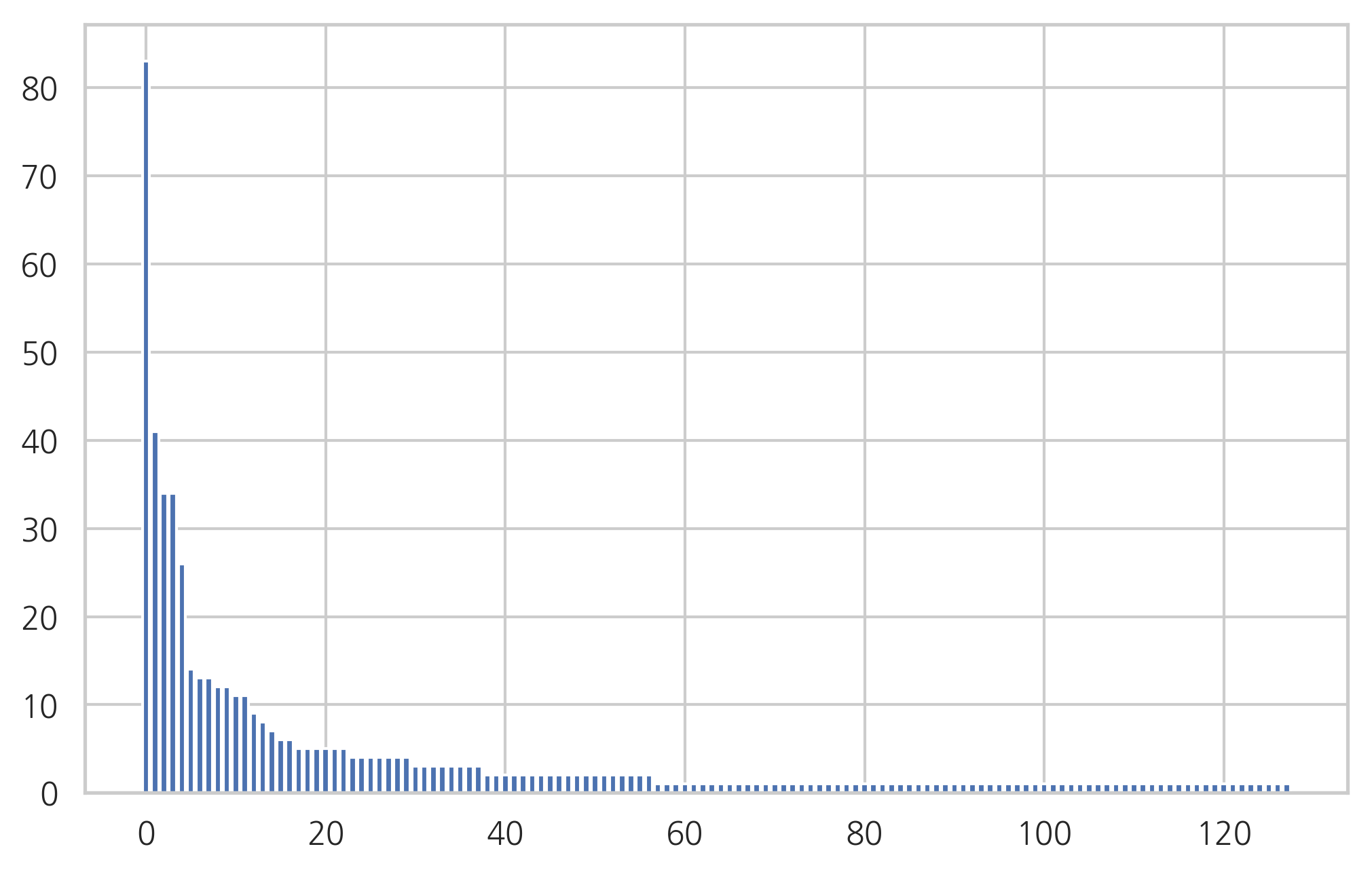
pprint(list(zip(feature_name, count))[:10])
[('컨테이너', 83),
 ('도커', 41),
 ('명령', 34),
 ('이미지', 34),
 ('사용', 26),
 ('가동', 14),
 ('중지', 13),
 ('mingw64', 13),
 ('다음', 12),
 ('삭제', 12)]