5.1 분류용 예제 데이터#
여기에서는 사이킷런 패키지에서 제공하는 분류용 예제 데이터의 일부를 소개한다. 이 데이터들을 살펴보면서 분류 모형에 대한 기초적인 공부를 시작한다.
붓꽃 데이터#
붓꽃 데이터는 통계학자 피셔(R.A Fisher)의 붓꽃의 분류 연구에 기반한 데이터다. load_iris() 명령으로 로드한다. 데이터는 다음과 같이 구성되어 있다.
타겟 데이터
setosa, versicolor, virginica의 세가지 붓꽃 종(species)
특징 데이터
꽃받침 길이(Sepal Length)
꽃받침 폭(Sepal Width)
꽃잎 길이(Petal Length)
꽃잎 폭(Petal Width)
좀 더 자세한 내용은 load_iris() 명령으로 로드한 데이터의 DESCR 속성으로 알 수 있다.
from sklearn.datasets import load_iris
iris = load_iris()
print(iris.DESCR)
.. _iris_dataset:

Iris plants dataset
--------------------

**Data Set Characteristics:**

    :Number of Instances: 150 (50 in each of three classes)
    :Number of Attributes: 4 numeric, predictive attributes and the class
    :Attribute Information:
        - sepal length in cm
        - sepal width in cm
        - petal length in cm
        - petal width in cm
        - class:
                - Iris-Setosa
                - Iris-Versicolour
                - Iris-Virginica

    :Summary Statistics:

    ============== ==== ==== ======= ===== ====================
                    Min  Max   Mean    SD   Class Correlation
    ============== ==== ==== ======= ===== ====================
    sepal length:   4.3  7.9   5.84   0.83    0.7826
    sepal width:    2.0  4.4   3.05   0.43   -0.4194
    petal length:   1.0  6.9   3.76   1.76    0.9490  (high!)
    petal width:    0.1  2.5   1.20   0.76    0.9565  (high!)
    ============== ==== ==== ======= ===== ====================

    :Missing Attribute Values: None
    :Class Distribution: 33.3% for each of 3 classes.
    :Creator: R.A. Fisher
    :Donor: Michael Marshall (MARSHALL%PLU@io.arc.nasa.gov)
    :Date: July, 1988

The famous Iris database, first used by Sir R.A. Fisher. The dataset is taken
from Fisher's paper. Note that it's the same as in R, but not as in the UCI
Machine Learning Repository, which has two wrong data points.

This is perhaps the best known database to be found in the
pattern recognition literature.  Fisher's paper is a classic in the field and
is referenced frequently to this day.  (See Duda & Hart, for example.)  The
data set contains 3 classes of 50 instances each, where each class refers to a
type of iris plant.  One class is linearly separable from the other 2; the
latter are NOT linearly separable from each other.

.. topic:: References

   - Fisher, R.A. "The use of multiple measurements in taxonomic problems"
     Annual Eugenics, 7, Part II, 179-188 (1936); also in "Contributions to
     Mathematical Statistics" (John Wiley, NY, 1950).
   - Duda, R.O., & Hart, P.E. (1973) Pattern Classification and Scene Analysis.
     (Q327.D83) John Wiley & Sons.  ISBN 0-471-22361-1.  See page 218.
   - Dasarathy, B.V. (1980) "Nosing Around the Neighborhood: A New System
     Structure and Classification Rule for Recognition in Partially Exposed
     Environments".  IEEE Transactions on Pattern Analysis and Machine
     Intelligence, Vol. PAMI-2, No. 1, 67-71.
   - Gates, G.W. (1972) "The Reduced Nearest Neighbor Rule".  IEEE Transactions
     on Information Theory, May 1972, 431-433.
   - See also: 1988 MLC Proceedings, 54-64.  Cheeseman et al"s AUTOCLASS II
     conceptual clustering system finds 3 classes in the data.
   - Many, many more ...
Pandas패키지로 데이터프레임을 만들어 일부 데이터를 살펴본다.
df = pd.DataFrame(iris.data, columns=iris.feature_names)
sy = pd.Series(iris.target, dtype="category")
sy = sy.cat.rename_categories(iris.target_names)
df['species'] = sy
df.tail()
| sepal length (cm) | sepal width (cm) | petal length (cm) | petal width (cm) | species | |
|---|---|---|---|---|---|
| 145 | 6.7 | 3.0 | 5.2 | 2.3 | virginica |
| 146 | 6.3 | 2.5 | 5.0 | 1.9 | virginica |
| 147 | 6.5 | 3.0 | 5.2 | 2.0 | virginica |
| 148 | 6.2 | 3.4 | 5.4 | 2.3 | virginica |
| 149 | 5.9 | 3.0 | 5.1 | 1.8 | virginica |
각 특징값의 분포와 상관관계를 히스토그램과 스캐터플롯으로 나타내면 다음과 같다.
sns.pairplot(df, hue="species")
plt.show()
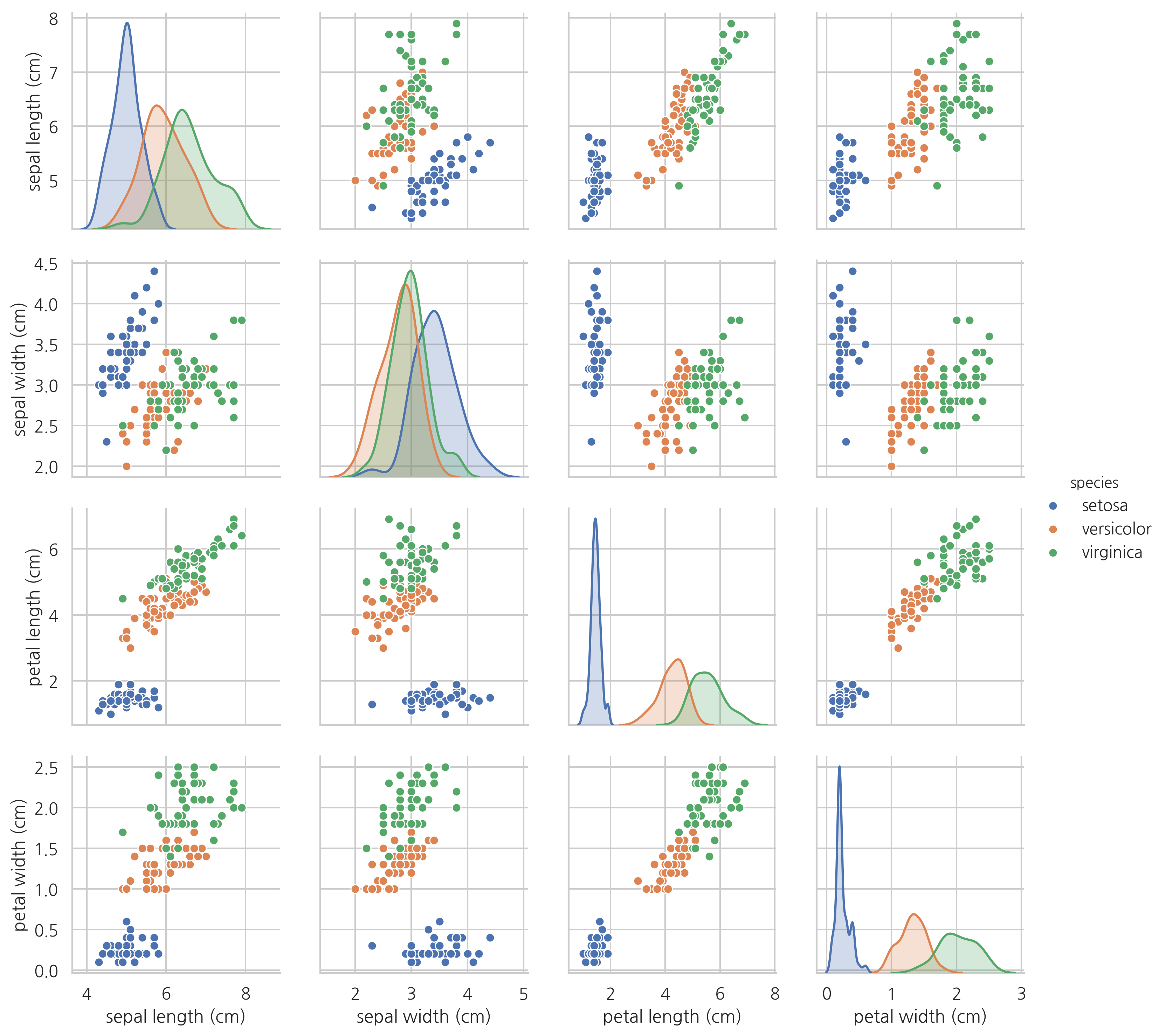
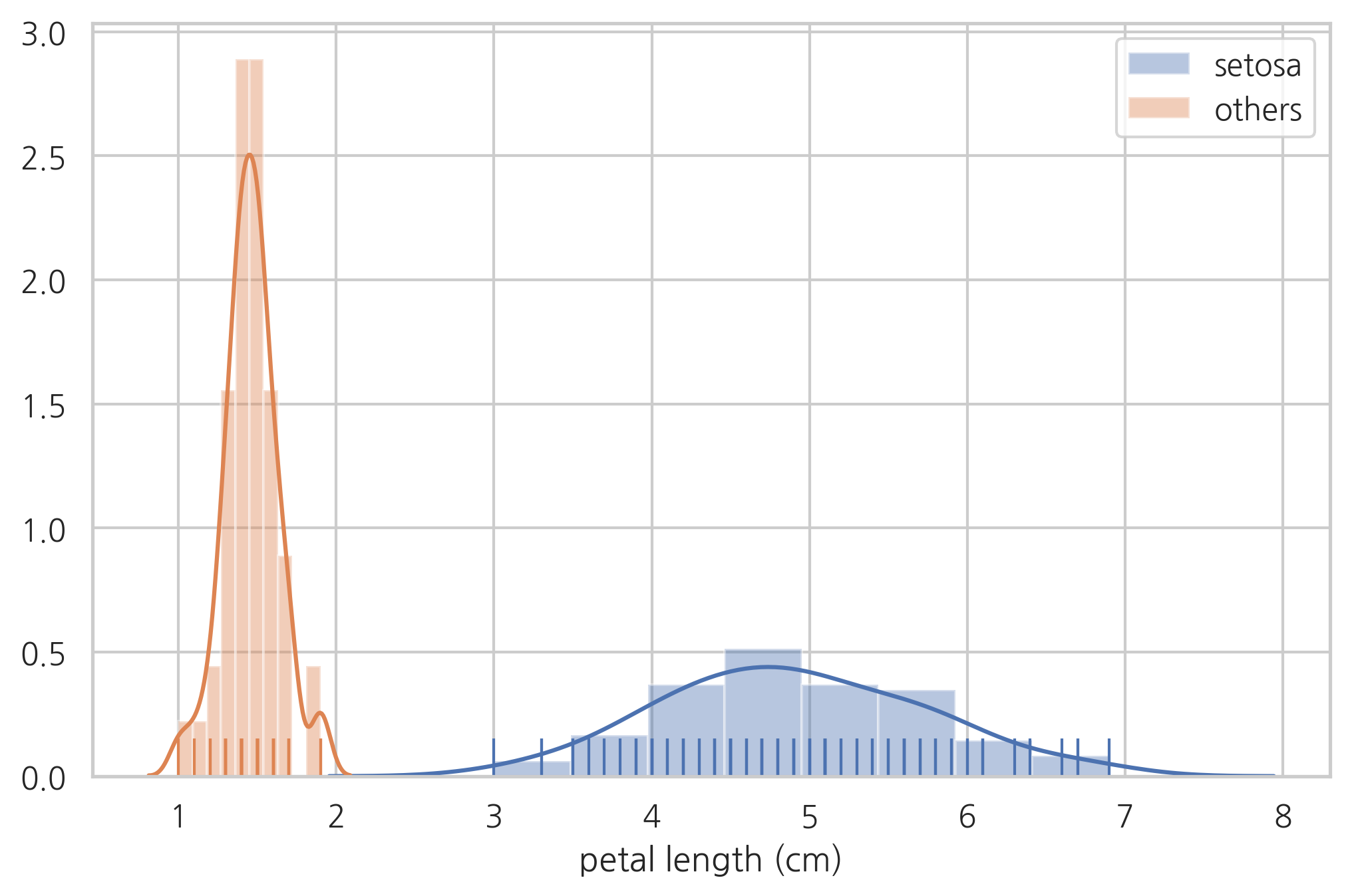
이 분포를 잘 살펴보면 꽃잎의 길이만으로도 세토사와 다른 종을 분류할 수 있다는 것을 알 수 있다.
sns.distplot(df[df.species != "setosa"]["petal length (cm)"], hist=True, rug=True, label="setosa")
sns.distplot(df[df.species == "setosa"]["petal length (cm)"], hist=True, rug=True, label="others")
plt.legend()
plt.show()
연습 문제 1#
꽃잎 길이의 기준값(thresh)이 얼마이면 세토사와 다른 종을 완벽하게 구분할 수 있는가?
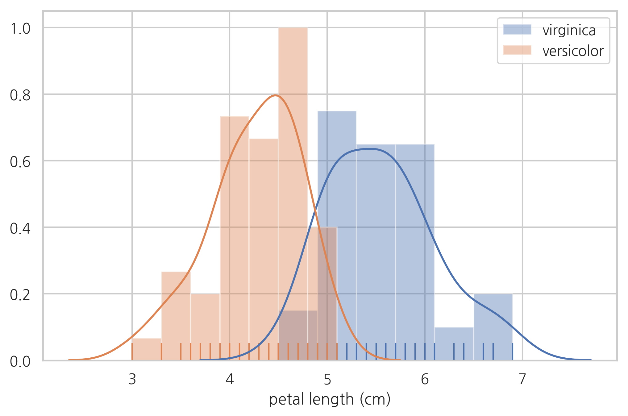
하지만 베르시칼라와 버지니카는 이 방법으로 완벽한 구분이 불가능하다.
sns.distplot(df[df.species == "virginica"]["petal length (cm)"], hist=True, rug=True, label="virginica")
sns.distplot(df[df.species == "versicolor"]["petal length (cm)"], hist=True, rug=True, label="versicolor")
plt.legend()
plt.show()
연습 문제 2#
(1) 가장 적합한 꽃잎 길이의 기준값(thresh)을 생각하고 이 값을 이용하여 베르시칼라와 버지니카를 분류하라.
(2) 위 방법에 따라서 분류하였을 때 잘못 분류된 표본의 갯수는 몇개인가?
와인 데이터#
와인의 화학 조성을 사용하여 와인의 종류를 예측하기 위한 데이터이다. load_wine() 명령으로 로드하며 다음과 같이 구성되어 있다.
타겟 데이터
와인의 종류 0, 1, 2의 세가지 값
특징 데이터
알콜(Alcohol)
말산(Malic acid)
회분(Ash)
회분의 알칼리도(Alcalinity of ash)
마그네슘(Magnesium)
총 폴리페놀(Total phenols)
플라보노이드 폴리페놀(Flavanoids)
비 플라보노이드 폴리페놀(Nonflavanoid phenols)
프로안토시아닌(Proanthocyanins)
색상의 강도(Color intensity)
색상(Hue)
희석 와인의 OD280/OD315 비율 (OD280/OD315 of diluted wines)
프롤린(Proline)
from sklearn.datasets import load_wine
wine = load_wine()
print(wine.DESCR)
.. _wine_dataset:

Wine recognition dataset
------------------------

**Data Set Characteristics:**

    :Number of Instances: 178 (50 in each of three classes)
    :Number of Attributes: 13 numeric, predictive attributes and the class
    :Attribute Information:
 		- Alcohol
 		- Malic acid
 		- Ash
		- Alcalinity of ash
 		- Magnesium
		- Total phenols
 		- Flavanoids
 		- Nonflavanoid phenols
 		- Proanthocyanins
		- Color intensity
 		- Hue
 		- OD280/OD315 of diluted wines
 		- Proline

    - class:
            - class_0
            - class_1
            - class_2

    :Summary Statistics:

    ============================= ==== ===== ======= =====
                                   Min   Max   Mean     SD
    ============================= ==== ===== ======= =====
    Alcohol:                      11.0  14.8    13.0   0.8
    Malic Acid:                   0.74  5.80    2.34  1.12
    Ash:                          1.36  3.23    2.36  0.27
    Alcalinity of Ash:            10.6  30.0    19.5   3.3
    Magnesium:                    70.0 162.0    99.7  14.3
    Total Phenols:                0.98  3.88    2.29  0.63
    Flavanoids:                   0.34  5.08    2.03  1.00
    Nonflavanoid Phenols:         0.13  0.66    0.36  0.12
    Proanthocyanins:              0.41  3.58    1.59  0.57
    Colour Intensity:              1.3  13.0     5.1   2.3
    Hue:                          0.48  1.71    0.96  0.23
    OD280/OD315 of diluted wines: 1.27  4.00    2.61  0.71
    Proline:                       278  1680     746   315
    ============================= ==== ===== ======= =====

    :Missing Attribute Values: None
    :Class Distribution: class_0 (59), class_1 (71), class_2 (48)
    :Creator: R.A. Fisher
    :Donor: Michael Marshall (MARSHALL%PLU@io.arc.nasa.gov)
    :Date: July, 1988

This is a copy of UCI ML Wine recognition datasets.
https://archive.ics.uci.edu/ml/machine-learning-databases/wine/wine.data

The data is the results of a chemical analysis of wines grown in the same
region in Italy by three different cultivators. There are thirteen different
measurements taken for different constituents found in the three types of
wine.

Original Owners:

Forina, M. et al, PARVUS -
An Extendible Package for Data Exploration, Classification and Correlation.
Institute of Pharmaceutical and Food Analysis and Technologies,
Via Brigata Salerno, 16147 Genoa, Italy.

Citation:

Lichman, M. (2013). UCI Machine Learning Repository
[http://archive.ics.uci.edu/ml]. Irvine, CA: University of California,
School of Information and Computer Science.

.. topic:: References

  (1) S. Aeberhard, D. Coomans and O. de Vel,
  Comparison of Classifiers in High Dimensional Settings,
  Tech. Rep. no. 92-02, (1992), Dept. of Computer Science and Dept. of
  Mathematics and Statistics, James Cook University of North Queensland.
  (Also submitted to Technometrics).

  The data was used with many others for comparing various
  classifiers. The classes are separable, though only RDA
  has achieved 100% correct classification.
  (RDA : 100%, QDA 99.4%, LDA 98.9%, 1NN 96.1% (z-transformed data))
  (All results using the leave-one-out technique)

  (2) S. Aeberhard, D. Coomans and O. de Vel,
  "THE CLASSIFICATION PERFORMANCE OF RDA"
  Tech. Rep. no. 92-01, (1992), Dept. of Computer Science and Dept. of
  Mathematics and Statistics, James Cook University of North Queensland.
  (Also submitted to Journal of Chemometrics).
df = pd.DataFrame(wine.data, columns=wine.feature_names)
sy = pd.Series(wine.target, dtype="category")
sy = sy.cat.rename_categories(wine.target_names)
df['class'] = sy
df.tail()
| alcohol | malic_acid | ash | alcalinity_of_ash | magnesium | total_phenols | flavanoids | nonflavanoid_phenols | proanthocyanins | color_intensity | hue | od280/od315_of_diluted_wines | proline | class | |
|---|---|---|---|---|---|---|---|---|---|---|---|---|---|---|
| 173 | 13.71 | 5.65 | 2.45 | 20.5 | 95.0 | 1.68 | 0.61 | 0.52 | 1.06 | 7.7 | 0.64 | 1.74 | 740.0 | class_2 |
| 174 | 13.40 | 3.91 | 2.48 | 23.0 | 102.0 | 1.80 | 0.75 | 0.43 | 1.41 | 7.3 | 0.70 | 1.56 | 750.0 | class_2 |
| 175 | 13.27 | 4.28 | 2.26 | 20.0 | 120.0 | 1.59 | 0.69 | 0.43 | 1.35 | 10.2 | 0.59 | 1.56 | 835.0 | class_2 |
| 176 | 13.17 | 2.59 | 2.37 | 20.0 | 120.0 | 1.65 | 0.68 | 0.53 | 1.46 | 9.3 | 0.60 | 1.62 | 840.0 | class_2 |
| 177 | 14.13 | 4.10 | 2.74 | 24.5 | 96.0 | 2.05 | 0.76 | 0.56 | 1.35 | 9.2 | 0.61 | 1.60 | 560.0 | class_2 |
일부 특징값의 분포와 상관관계를 히스토그램과 스캐터플롯으로 나타내면 다음과 같다.
sns.pairplot(vars=["alcohol", "alcalinity_of_ash", "total_phenols", "flavanoids"],
             hue="class", data=df)
plt.show()
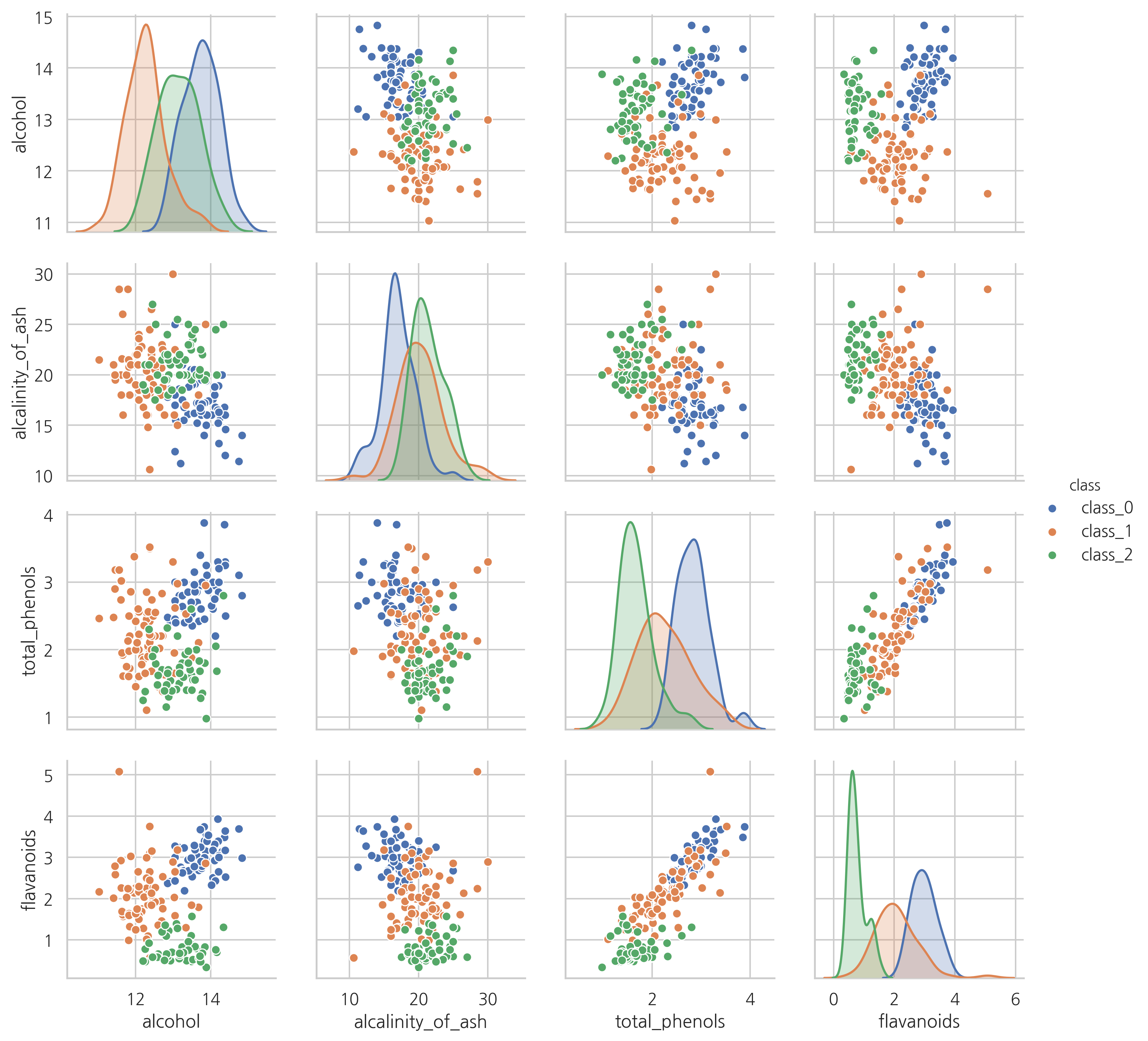
연습 문제 3#
위 시각화 결과에서 어떤 특징값을 사용하면 두 개의 클래스를 완벽하게 구분할 수 있다는 것을 알 수 있다. 어떤 특징값이고 어떤 클래스를 구분할 수 있는가?
유방암 진단 데이터#
load_breast_cancer 명령은 유방암(breast cancer) 진단 데이터를 제공한다. 유방암 진단 사진으로부터 측정한 종양(tumar)의 특징값을 사용하여 종양이 양성(benign)인지 악성(malignant)인지를 판별한다.
from sklearn.datasets import load_breast_cancer
cancer = load_breast_cancer()
print(cancer.DESCR)
.. _breast_cancer_dataset:

Breast cancer wisconsin (diagnostic) dataset
--------------------------------------------

**Data Set Characteristics:**

    :Number of Instances: 569

    :Number of Attributes: 30 numeric, predictive attributes and the class

    :Attribute Information:
        - radius (mean of distances from center to points on the perimeter)
        - texture (standard deviation of gray-scale values)
        - perimeter
        - area
        - smoothness (local variation in radius lengths)
        - compactness (perimeter^2 / area - 1.0)
        - concavity (severity of concave portions of the contour)
        - concave points (number of concave portions of the contour)
        - symmetry
        - fractal dimension ("coastline approximation" - 1)

        The mean, standard error, and "worst" or largest (mean of the three
        largest values) of these features were computed for each image,
        resulting in 30 features.  For instance, field 3 is Mean Radius, field
        13 is Radius SE, field 23 is Worst Radius.

        - class:
                - WDBC-Malignant
                - WDBC-Benign

    :Summary Statistics:

    ===================================== ====== ======
                                           Min    Max
    ===================================== ====== ======
    radius (mean):                        6.981  28.11
    texture (mean):                       9.71   39.28
    perimeter (mean):                     43.79  188.5
    area (mean):                          143.5  2501.0
    smoothness (mean):                    0.053  0.163
    compactness (mean):                   0.019  0.345
    concavity (mean):                     0.0    0.427
    concave points (mean):                0.0    0.201
    symmetry (mean):                      0.106  0.304
    fractal dimension (mean):             0.05   0.097
    radius (standard error):              0.112  2.873
    texture (standard error):             0.36   4.885
    perimeter (standard error):           0.757  21.98
    area (standard error):                6.802  542.2
    smoothness (standard error):          0.002  0.031
    compactness (standard error):         0.002  0.135
    concavity (standard error):           0.0    0.396
    concave points (standard error):      0.0    0.053
    symmetry (standard error):            0.008  0.079
    fractal dimension (standard error):   0.001  0.03
    radius (worst):                       7.93   36.04
    texture (worst):                      12.02  49.54
    perimeter (worst):                    50.41  251.2
    area (worst):                         185.2  4254.0
    smoothness (worst):                   0.071  0.223
    compactness (worst):                  0.027  1.058
    concavity (worst):                    0.0    1.252
    concave points (worst):               0.0    0.291
    symmetry (worst):                     0.156  0.664
    fractal dimension (worst):            0.055  0.208
    ===================================== ====== ======

    :Missing Attribute Values: None

    :Class Distribution: 212 - Malignant, 357 - Benign

    :Creator:  Dr. William H. Wolberg, W. Nick Street, Olvi L. Mangasarian

    :Donor: Nick Street

    :Date: November, 1995

This is a copy of UCI ML Breast Cancer Wisconsin (Diagnostic) datasets.
https://goo.gl/U2Uwz2

Features are computed from a digitized image of a fine needle
aspirate (FNA) of a breast mass.  They describe
characteristics of the cell nuclei present in the image.

Separating plane described above was obtained using
Multisurface Method-Tree (MSM-T) [K. P. Bennett, "Decision Tree
Construction Via Linear Programming." Proceedings of the 4th
Midwest Artificial Intelligence and Cognitive Science Society,
pp. 97-101, 1992], a classification method which uses linear
programming to construct a decision tree.  Relevant features
were selected using an exhaustive search in the space of 1-4
features and 1-3 separating planes.

The actual linear program used to obtain the separating plane
in the 3-dimensional space is that described in:
[K. P. Bennett and O. L. Mangasarian: "Robust Linear
Programming Discrimination of Two Linearly Inseparable Sets",
Optimization Methods and Software 1, 1992, 23-34].

This database is also available through the UW CS ftp server:

ftp ftp.cs.wisc.edu
cd math-prog/cpo-dataset/machine-learn/WDBC/

.. topic:: References

   - W.N. Street, W.H. Wolberg and O.L. Mangasarian. Nuclear feature extraction
     for breast tumor diagnosis. IS&T/SPIE 1993 International Symposium on
     Electronic Imaging: Science and Technology, volume 1905, pages 861-870,
     San Jose, CA, 1993.
   - O.L. Mangasarian, W.N. Street and W.H. Wolberg. Breast cancer diagnosis and
     prognosis via linear programming. Operations Research, 43(4), pages 570-577,
     July-August 1995.
   - W.H. Wolberg, W.N. Street, and O.L. Mangasarian. Machine learning techniques
     to diagnose breast cancer from fine-needle aspirates. Cancer Letters 77 (1994)
     163-171.
df = pd.DataFrame(cancer.data, columns=cancer.feature_names)
sy = pd.Series(cancer.target, dtype="category")
sy = sy.cat.rename_categories(cancer.target_names)
df['class'] = sy
df.tail()
| mean radius | mean texture | mean perimeter | mean area | mean smoothness | mean compactness | mean concavity | mean concave points | mean symmetry | mean fractal dimension | ... | worst texture | worst perimeter | worst area | worst smoothness | worst compactness | worst concavity | worst concave points | worst symmetry | worst fractal dimension | class | |
|---|---|---|---|---|---|---|---|---|---|---|---|---|---|---|---|---|---|---|---|---|---|
| 564 | 21.56 | 22.39 | 142.00 | 1479.0 | 0.11100 | 0.11590 | 0.24390 | 0.13890 | 0.1726 | 0.05623 | ... | 26.40 | 166.10 | 2027.0 | 0.14100 | 0.21130 | 0.4107 | 0.2216 | 0.2060 | 0.07115 | malignant |
| 565 | 20.13 | 28.25 | 131.20 | 1261.0 | 0.09780 | 0.10340 | 0.14400 | 0.09791 | 0.1752 | 0.05533 | ... | 38.25 | 155.00 | 1731.0 | 0.11660 | 0.19220 | 0.3215 | 0.1628 | 0.2572 | 0.06637 | malignant |
| 566 | 16.60 | 28.08 | 108.30 | 858.1 | 0.08455 | 0.10230 | 0.09251 | 0.05302 | 0.1590 | 0.05648 | ... | 34.12 | 126.70 | 1124.0 | 0.11390 | 0.30940 | 0.3403 | 0.1418 | 0.2218 | 0.07820 | malignant |
| 567 | 20.60 | 29.33 | 140.10 | 1265.0 | 0.11780 | 0.27700 | 0.35140 | 0.15200 | 0.2397 | 0.07016 | ... | 39.42 | 184.60 | 1821.0 | 0.16500 | 0.86810 | 0.9387 | 0.2650 | 0.4087 | 0.12400 | malignant |
| 568 | 7.76 | 24.54 | 47.92 | 181.0 | 0.05263 | 0.04362 | 0.00000 | 0.00000 | 0.1587 | 0.05884 | ... | 30.37 | 59.16 | 268.6 | 0.08996 | 0.06444 | 0.0000 | 0.0000 | 0.2871 | 0.07039 | benign |
5 rows × 31 columns
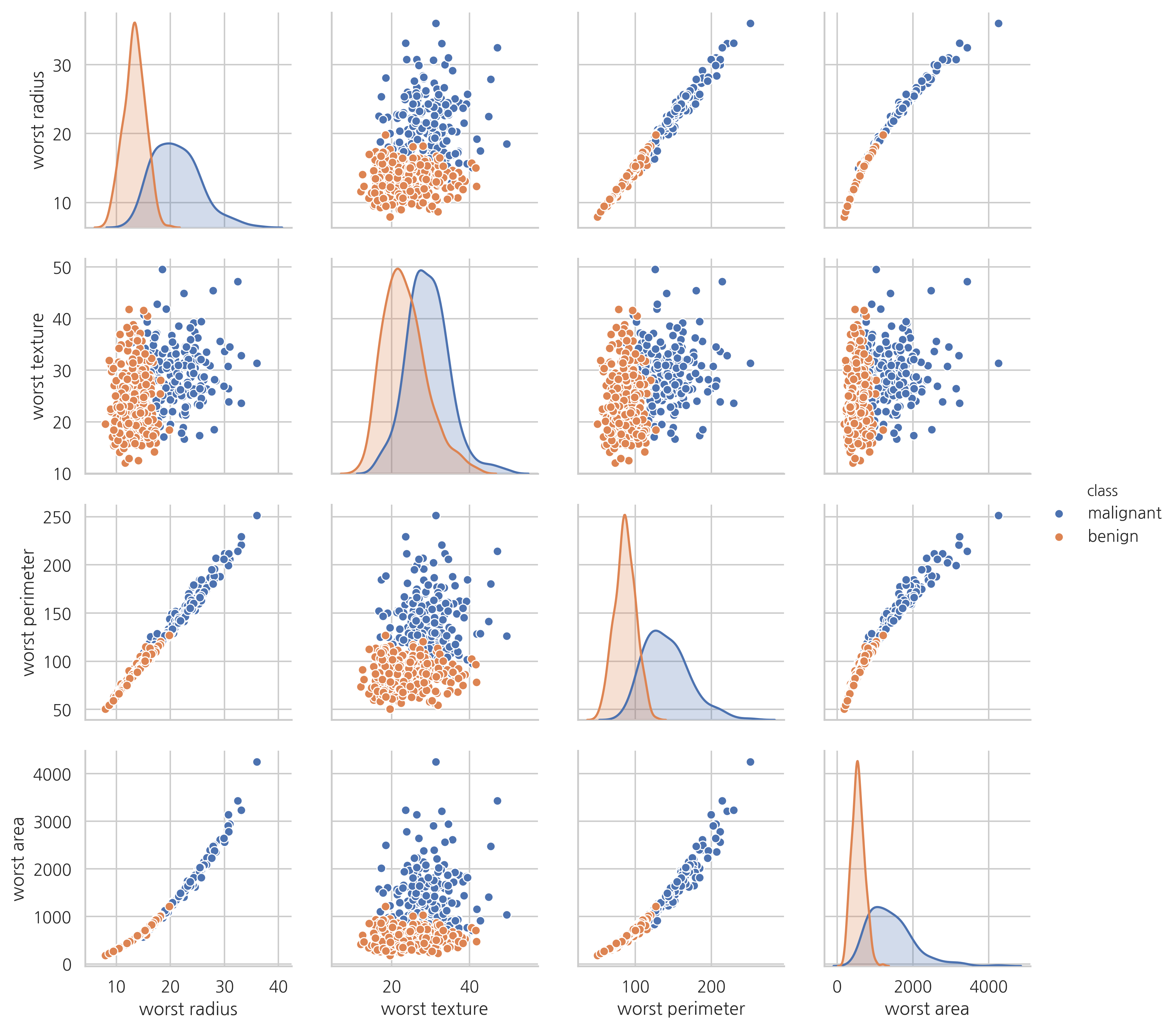
sns.pairplot(vars=["worst radius", "worst texture", "worst perimeter", "worst area"],
             hue="class", data=df)
plt.show()
대표 수종 데이터#
대표 수종 데이터는 미국 삼림을 30×30m 영역으로 나누어 각 영역의 특징으로부터 대표적인 나무의 종류(species of tree)을 예측하기위한 데이터이다. 수종은 7종류이지만 특징 데이터가 54종류, 표본 데이터의 갯수가 581,012개에 달하는 대규모 데이터이다.
from sklearn.datasets import fetch_covtype
covtype = fetch_covtype()
print(covtype.DESCR)
.. _covtype_dataset:

Forest covertypes
-----------------

The samples in this dataset correspond to 30×30m patches of forest in the US,
collected for the task of predicting each patch's cover type,
i.e. the dominant species of tree.
There are seven covertypes, making this a multiclass classification problem.
Each sample has 54 features, described on the
`dataset's homepage <http://archive.ics.uci.edu/ml/datasets/Covertype>`__.
Some of the features are boolean indicators,
while others are discrete or continuous measurements.

**Data Set Characteristics:**

    =================   ============
    Classes                        7
    Samples total             581012
    Dimensionality                54
    Features                     int
    =================   ============

:func:`sklearn.datasets.fetch_covtype` will load the covertype dataset;
it returns a dictionary-like object
with the feature matrix in the ``data`` member
and the target values in ``target``.
The dataset will be downloaded from the web if necessary.
df = pd.DataFrame(covtype.data,
                  columns=["x{:02d}".format(i + 1) for i in range(covtype.data.shape[1])],
                  dtype=int)
sy = pd.Series(covtype.target, dtype="category")
df['covtype'] = sy
df.tail()
| x01 | x02 | x03 | x04 | x05 | x06 | x07 | x08 | x09 | x10 | ... | x46 | x47 | x48 | x49 | x50 | x51 | x52 | x53 | x54 | covtype | |
|---|---|---|---|---|---|---|---|---|---|---|---|---|---|---|---|---|---|---|---|---|---|
| 581007 | 2396 | 153 | 20 | 85 | 17 | 108 | 240 | 237 | 118 | 837 | ... | 0 | 0 | 0 | 0 | 0 | 0 | 0 | 0 | 0 | 3 |
| 581008 | 2391 | 152 | 19 | 67 | 12 | 95 | 240 | 237 | 119 | 845 | ... | 0 | 0 | 0 | 0 | 0 | 0 | 0 | 0 | 0 | 3 |
| 581009 | 2386 | 159 | 17 | 60 | 7 | 90 | 236 | 241 | 130 | 854 | ... | 0 | 0 | 0 | 0 | 0 | 0 | 0 | 0 | 0 | 3 |
| 581010 | 2384 | 170 | 15 | 60 | 5 | 90 | 230 | 245 | 143 | 864 | ... | 0 | 0 | 0 | 0 | 0 | 0 | 0 | 0 | 0 | 3 |
| 581011 | 2383 | 165 | 13 | 60 | 4 | 67 | 231 | 244 | 141 | 875 | ... | 0 | 0 | 0 | 0 | 0 | 0 | 0 | 0 | 0 | 3 |
5 rows × 55 columns
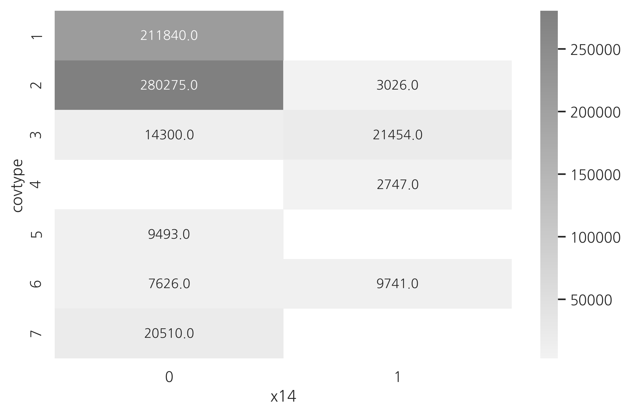
각 특징 데이터가 가지는 값의 종류를 보면 1번부터 10번 특징은 실수값이고 11번부터 54번 특징은 이진 카테고리값이라는 것을 알 수 있다.
pd.DataFrame(df.nunique()).T
| x01 | x02 | x03 | x04 | x05 | x06 | x07 | x08 | x09 | x10 | ... | x46 | x47 | x48 | x49 | x50 | x51 | x52 | x53 | x54 | covtype | |
|---|---|---|---|---|---|---|---|---|---|---|---|---|---|---|---|---|---|---|---|---|---|
| 0 | 1978 | 361 | 67 | 551 | 700 | 5785 | 207 | 185 | 255 | 5827 | ... | 2 | 2 | 2 | 2 | 2 | 2 | 2 | 2 | 2 | 7 |
1 rows × 55 columns
따라서 이 값을 카테고리 형태로 바꾼다.
df.iloc[:, 10:54] = df.iloc[:, 10:54].astype('category')
다음 플롯은 카테고리값에 따라 “x14” 특징의 값이 어떻게 변하는지 나타낸 것이다. “x14” 특징이 0인가 1인가를 사용하면 1, 5, 7번 클래스와 4번 클래스는 완벽하게 분류할 수 있다는 것을 알 수 있다.
df_count = df.pivot_table(index="covtype", columns="x14", aggfunc="size")
sns.heatmap(df_count, cmap=sns.light_palette("gray", as_cmap=True), annot=True, fmt="0")
plt.show()
뉴스 그룹 텍스트 데이터#
20개의 뉴스 그룹 문서 데이터. fetch_20newsgroups() 명령으로 로드하며 다음과 같이 구성되어 있다.
타겟 데이터
문서가 속한 뉴스 그룹
특징 데이터
문서 텍스트
from sklearn.datasets import fetch_20newsgroups
newsgroups = fetch_20newsgroups(subset='all')
print(newsgroups.DESCR)
.. _20newsgroups_dataset:

The 20 newsgroups text dataset
------------------------------

The 20 newsgroups dataset comprises around 18000 newsgroups posts on
20 topics split in two subsets: one for training (or development)
and the other one for testing (or for performance evaluation). The split
between the train and test set is based upon a messages posted before
and after a specific date.

This module contains two loaders. The first one,
:func:`sklearn.datasets.fetch_20newsgroups`,
returns a list of the raw texts that can be fed to text feature
extractors such as :class:`sklearn.feature_extraction.text.CountVectorizer`
with custom parameters so as to extract feature vectors.
The second one, :func:`sklearn.datasets.fetch_20newsgroups_vectorized`,
returns ready-to-use features, i.e., it is not necessary to use a feature
extractor.

**Data Set Characteristics:**

    =================   ==========
    Classes                     20
    Samples total            18846
    Dimensionality               1
    Features                  text
    =================   ==========

Usage
~~~~~

The :func:`sklearn.datasets.fetch_20newsgroups` function is a data
fetching / caching functions that downloads the data archive from
the original `20 newsgroups website`_, extracts the archive contents
in the ``~/scikit_learn_data/20news_home`` folder and calls the
:func:`sklearn.datasets.load_files` on either the training or
testing set folder, or both of them::

  >>> from sklearn.datasets import fetch_20newsgroups
  >>> newsgroups_train = fetch_20newsgroups(subset='train')

  >>> from pprint import pprint
  >>> pprint(list(newsgroups_train.target_names))
  ['alt.atheism',
   'comp.graphics',
   'comp.os.ms-windows.misc',
   'comp.sys.ibm.pc.hardware',
   'comp.sys.mac.hardware',
   'comp.windows.x',
   'misc.forsale',
   'rec.autos',
   'rec.motorcycles',
   'rec.sport.baseball',
   'rec.sport.hockey',
   'sci.crypt',
   'sci.electronics',
   'sci.med',
   'sci.space',
   'soc.religion.christian',
   'talk.politics.guns',
   'talk.politics.mideast',
   'talk.politics.misc',
   'talk.religion.misc']

The real data lies in the ``filenames`` and ``target`` attributes. The target
attribute is the integer index of the category::

  >>> newsgroups_train.filenames.shape
  (11314,)
  >>> newsgroups_train.target.shape
  (11314,)
  >>> newsgroups_train.target[:10]
  array([ 7,  4,  4,  1, 14, 16, 13,  3,  2,  4])

It is possible to load only a sub-selection of the categories by passing the
list of the categories to load to the
:func:`sklearn.datasets.fetch_20newsgroups` function::

  >>> cats = ['alt.atheism', 'sci.space']
  >>> newsgroups_train = fetch_20newsgroups(subset='train', categories=cats)

  >>> list(newsgroups_train.target_names)
  ['alt.atheism', 'sci.space']
  >>> newsgroups_train.filenames.shape
  (1073,)
  >>> newsgroups_train.target.shape
  (1073,)
  >>> newsgroups_train.target[:10]
  array([0, 1, 1, 1, 0, 1, 1, 0, 0, 0])

Converting text to vectors
~~~~~~~~~~~~~~~~~~~~~~~~~~

In order to feed predictive or clustering models with the text data,
one first need to turn the text into vectors of numerical values suitable
for statistical analysis. This can be achieved with the utilities of the
``sklearn.feature_extraction.text`` as demonstrated in the following
example that extract `TF-IDF`_ vectors of unigram tokens
from a subset of 20news::

  >>> from sklearn.feature_extraction.text import TfidfVectorizer
  >>> categories = ['alt.atheism', 'talk.religion.misc',
  ...               'comp.graphics', 'sci.space']
  >>> newsgroups_train = fetch_20newsgroups(subset='train',
  ...                                       categories=categories)
  >>> vectorizer = TfidfVectorizer()
  >>> vectors = vectorizer.fit_transform(newsgroups_train.data)
  >>> vectors.shape
  (2034, 34118)

The extracted TF-IDF vectors are very sparse, with an average of 159 non-zero
components by sample in a more than 30000-dimensional space
(less than .5% non-zero features)::

  >>> vectors.nnz / float(vectors.shape[0])       # doctest: +ELLIPSIS
  159.01327...

:func:`sklearn.datasets.fetch_20newsgroups_vectorized` is a function which
returns ready-to-use token counts features instead of file names.

.. _`20 newsgroups website`: http://people.csail.mit.edu/jrennie/20Newsgroups/
.. _`TF-IDF`: https://en.wikipedia.org/wiki/Tf-idf


Filtering text for more realistic training
~~~~~~~~~~~~~~~~~~~~~~~~~~~~~~~~~~~~~~~~~~

It is easy for a classifier to overfit on particular things that appear in the
20 Newsgroups data, such as newsgroup headers. Many classifiers achieve very
high F-scores, but their results would not generalize to other documents that
aren't from this window of time.

For example, let's look at the results of a multinomial Naive Bayes classifier,
which is fast to train and achieves a decent F-score::

  >>> from sklearn.naive_bayes import MultinomialNB
  >>> from sklearn import metrics
  >>> newsgroups_test = fetch_20newsgroups(subset='test',
  ...                                      categories=categories)
  >>> vectors_test = vectorizer.transform(newsgroups_test.data)
  >>> clf = MultinomialNB(alpha=.01)
  >>> clf.fit(vectors, newsgroups_train.target)
  MultinomialNB(alpha=0.01, class_prior=None, fit_prior=True)

  >>> pred = clf.predict(vectors_test)
  >>> metrics.f1_score(newsgroups_test.target, pred, average='macro')  # doctest: +ELLIPSIS
  0.88213...

(The example :ref:`sphx_glr_auto_examples_text_plot_document_classification_20newsgroups.py` shuffles
the training and test data, instead of segmenting by time, and in that case
multinomial Naive Bayes gets a much higher F-score of 0.88. Are you suspicious
yet of what's going on inside this classifier?)

Let's take a look at what the most informative features are:

  >>> import numpy as np
  >>> def show_top10(classifier, vectorizer, categories):
  ...     feature_names = np.asarray(vectorizer.get_feature_names())
  ...     for i, category in enumerate(categories):
  ...         top10 = np.argsort(classifier.coef_[i])[-10:]
  ...         print("%s: %s" % (category, " ".join(feature_names[top10])))
  ...
  >>> show_top10(clf, vectorizer, newsgroups_train.target_names)
  alt.atheism: edu it and in you that is of to the
  comp.graphics: edu in graphics it is for and of to the
  sci.space: edu it that is in and space to of the
  talk.religion.misc: not it you in is that and to of the


You can now see many things that these features have overfit to:

- Almost every group is distinguished by whether headers such as
  ``NNTP-Posting-Host:`` and ``Distribution:`` appear more or less often.
- Another significant feature involves whether the sender is affiliated with
  a university, as indicated either by their headers or their signature.
- The word "article" is a significant feature, based on how often people quote
  previous posts like this: "In article [article ID], [name] <[e-mail address]>
  wrote:"
- Other features match the names and e-mail addresses of particular people who
  were posting at the time.

With such an abundance of clues that distinguish newsgroups, the classifiers
barely have to identify topics from text at all, and they all perform at the
same high level.

For this reason, the functions that load 20 Newsgroups data provide a
parameter called **remove**, telling it what kinds of information to strip out
of each file. **remove** should be a tuple containing any subset of
``('headers', 'footers', 'quotes')``, telling it to remove headers, signature
blocks, and quotation blocks respectively.

  >>> newsgroups_test = fetch_20newsgroups(subset='test',
  ...                                      remove=('headers', 'footers', 'quotes'),
  ...                                      categories=categories)
  >>> vectors_test = vectorizer.transform(newsgroups_test.data)
  >>> pred = clf.predict(vectors_test)
  >>> metrics.f1_score(pred, newsgroups_test.target, average='macro')  # doctest: +ELLIPSIS
  0.77310...

This classifier lost over a lot of its F-score, just because we removed
metadata that has little to do with topic classification.
It loses even more if we also strip this metadata from the training data:

  >>> newsgroups_train = fetch_20newsgroups(subset='train',
  ...                                       remove=('headers', 'footers', 'quotes'),
  ...                                       categories=categories)
  >>> vectors = vectorizer.fit_transform(newsgroups_train.data)
  >>> clf = MultinomialNB(alpha=.01)
  >>> clf.fit(vectors, newsgroups_train.target)
  MultinomialNB(alpha=0.01, class_prior=None, fit_prior=True)

  >>> vectors_test = vectorizer.transform(newsgroups_test.data)
  >>> pred = clf.predict(vectors_test)
  >>> metrics.f1_score(newsgroups_test.target, pred, average='macro')  # doctest: +ELLIPSIS
  0.76995...

Some other classifiers cope better with this harder version of the task. Try
running :ref:`sphx_glr_auto_examples_model_selection_grid_search_text_feature_extraction.py` with and without
the ``--filter`` option to compare the results.

.. topic:: Recommendation

  When evaluating text classifiers on the 20 Newsgroups data, you
  should strip newsgroup-related metadata. In scikit-learn, you can do this by
  setting ``remove=('headers', 'footers', 'quotes')``. The F-score will be
  lower because it is more realistic.

.. topic:: Examples

   * :ref:`sphx_glr_auto_examples_model_selection_grid_search_text_feature_extraction.py`

   * :ref:`sphx_glr_auto_examples_text_plot_document_classification_20newsgroups.py`
from pprint import pprint
pprint(list(newsgroups.target_names))
['alt.atheism',
 'comp.graphics',
 'comp.os.ms-windows.misc',
 'comp.sys.ibm.pc.hardware',
 'comp.sys.mac.hardware',
 'comp.windows.x',
 'misc.forsale',
 'rec.autos',
 'rec.motorcycles',
 'rec.sport.baseball',
 'rec.sport.hockey',
 'sci.crypt',
 'sci.electronics',
 'sci.med',
 'sci.space',
 'soc.religion.christian',
 'talk.politics.guns',
 'talk.politics.mideast',
 'talk.politics.misc',
 'talk.religion.misc']
print(newsgroups.data[1])
print("=" * 80)
print(newsgroups.target_names[newsgroups.target[1]])
From: mblawson@midway.ecn.uoknor.edu (Matthew B Lawson)
Subject: Which high-performance VLB video card?
Summary: Seek recommendations for VLB video card
Nntp-Posting-Host: midway.ecn.uoknor.edu
Organization: Engineering Computer Network, University of Oklahoma, Norman, OK, USA
Keywords: orchid, stealth, vlb
Lines: 21

  My brother is in the market for a high-performance video card that supports
VESA local bus with 1-2MB RAM.  Does anyone have suggestions/ideas on:

  - Diamond Stealth Pro Local Bus

  - Orchid Farenheit 1280

  - ATI Graphics Ultra Pro

  - Any other high-performance VLB card


Please post or email.  Thank you!

  - Matt

--
    |  Matthew B. Lawson <------------> (mblawson@essex.ecn.uoknor.edu)  |
  --+-- "Now I, Nebuchadnezzar, praise and exalt and glorify the King  --+--
    |   of heaven, because everything he does is right and all his ways  |
    |   are just." - Nebuchadnezzar, king of Babylon, 562 B.C.           |

================================================================================
comp.sys.ibm.pc.hardware
로이터 말뭉치#
로이터 말뭉치 데이터는 47,236개의 단어(vocalbulary)로 이루어진 804,414개의 문서를 103개의 클래스로 분류하기 위한 텍스트 데이터이다. TF-IDF 인코딩된 특징 데이터 행렬을 제공한다.
fetch_rcv1 명령으로 다운로드 받을 수 있다. 용량때문에 다운로드 시간이 오래 걸릴 수 있다.
from sklearn.datasets import fetch_rcv1
rcv = fetch_rcv1()
print(rcv.DESCR)
.. _rcv1_dataset:

RCV1 dataset
------------

Reuters Corpus Volume I (RCV1) is an archive of over 800,000 manually
categorized newswire stories made available by Reuters, Ltd. for research
purposes. The dataset is extensively described in [1]_.

**Data Set Characteristics:**

    ==============     =====================
    Classes                              103
    Samples total                     804414
    Dimensionality                     47236
    Features           real, between 0 and 1
    ==============     =====================

:func:`sklearn.datasets.fetch_rcv1` will load the following
version: RCV1-v2, vectors, full sets, topics multilabels::

    >>> from sklearn.datasets import fetch_rcv1
    >>> rcv1 = fetch_rcv1()

It returns a dictionary-like object, with the following attributes:

``data``:
The feature matrix is a scipy CSR sparse matrix, with 804414 samples and
47236 features. Non-zero values contains cosine-normalized, log TF-IDF vectors.
A nearly chronological split is proposed in [1]_: The first 23149 samples are
the training set. The last 781265 samples are the testing set. This follows
the official LYRL2004 chronological split. The array has 0.16% of non zero
values::

    >>> rcv1.data.shape
    (804414, 47236)

``target``:
The target values are stored in a scipy CSR sparse matrix, with 804414 samples
and 103 categories. Each sample has a value of 1 in its categories, and 0 in
others. The array has 3.15% of non zero values::

    >>> rcv1.target.shape
    (804414, 103)

``sample_id``:
Each sample can be identified by its ID, ranging (with gaps) from 2286
to 810596::

    >>> rcv1.sample_id[:3]
    array([2286, 2287, 2288], dtype=uint32)

``target_names``:
The target values are the topics of each sample. Each sample belongs to at
least one topic, and to up to 17 topics. There are 103 topics, each
represented by a string. Their corpus frequencies span five orders of
magnitude, from 5 occurrences for 'GMIL', to 381327 for 'CCAT'::

    >>> rcv1.target_names[:3].tolist()  # doctest: +SKIP
    ['E11', 'ECAT', 'M11']

The dataset will be downloaded from the `rcv1 homepage`_ if necessary.
The compressed size is about 656 MB.

.. _rcv1 homepage: http://jmlr.csail.mit.edu/papers/volume5/lewis04a/


.. topic:: References

    .. [1] Lewis, D. D., Yang, Y., Rose, T. G., & Li, F. (2004).
           RCV1: A new benchmark collection for text categorization research.
           The Journal of Machine Learning Research, 5, 361-397.
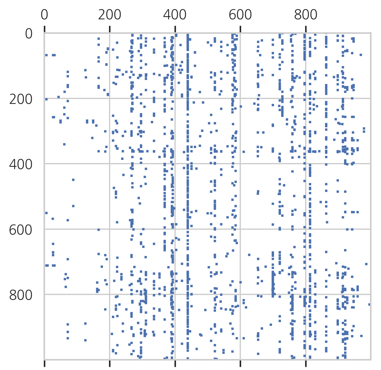
plt.spy(rcv.data[:1000, :1000], markersize=1)
plt.show()
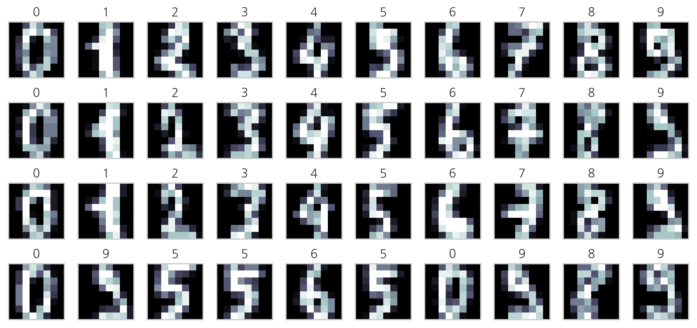
숫자 필기 이미지 데이터#
0부터 9까지의 숫자를 손으로 쓴 이미지 데이터. load_digits() 명령으로 로드한다. 각 이미지는 0부터 15까지의 명암을 가지는 8x8=64픽셀 해상도의 흑백 이미지이다.
from sklearn.datasets import load_digits
digits = load_digits()
print(digits.DESCR)
.. _digits_dataset:

Optical recognition of handwritten digits dataset
--------------------------------------------------

**Data Set Characteristics:**

    :Number of Instances: 5620
    :Number of Attributes: 64
    :Attribute Information: 8x8 image of integer pixels in the range 0..16.
    :Missing Attribute Values: None
    :Creator: E. Alpaydin (alpaydin '@' boun.edu.tr)
    :Date: July; 1998

This is a copy of the test set of the UCI ML hand-written digits datasets
http://archive.ics.uci.edu/ml/datasets/Optical+Recognition+of+Handwritten+Digits

The data set contains images of hand-written digits: 10 classes where
each class refers to a digit.

Preprocessing programs made available by NIST were used to extract
normalized bitmaps of handwritten digits from a preprinted form. From a
total of 43 people, 30 contributed to the training set and different 13
to the test set. 32x32 bitmaps are divided into nonoverlapping blocks of
4x4 and the number of on pixels are counted in each block. This generates
an input matrix of 8x8 where each element is an integer in the range
0..16. This reduces dimensionality and gives invariance to small
distortions.

For info on NIST preprocessing routines, see M. D. Garris, J. L. Blue, G.
T. Candela, D. L. Dimmick, J. Geist, P. J. Grother, S. A. Janet, and C.
L. Wilson, NIST Form-Based Handprint Recognition System, NISTIR 5469,
1994.

.. topic:: References

  - C. Kaynak (1995) Methods of Combining Multiple Classifiers and Their
    Applications to Handwritten Digit Recognition, MSc Thesis, Institute of
    Graduate Studies in Science and Engineering, Bogazici University.
  - E. Alpaydin, C. Kaynak (1998) Cascading Classifiers, Kybernetika.
  - Ken Tang and Ponnuthurai N. Suganthan and Xi Yao and A. Kai Qin.
    Linear dimensionalityreduction using relevance weighted LDA. School of
    Electrical and Electronic Engineering Nanyang Technological University.
    2005.
  - Claudio Gentile. A New Approximate Maximal Margin Classification
    Algorithm. NIPS. 2000.
np.random.seed(0)
N = 4
M = 10
fig = plt.figure(figsize=(10, 5))
plt.subplots_adjust(top=1, bottom=0, hspace=0, wspace=0.05)
for i in range(N):
    for j in range(M):
        k = i*M+j
        ax = fig.add_subplot(N, M, k+1)
        ax.imshow(digits.images[k], cmap=plt.cm.bone, interpolation="none")
        ax.grid(False)
        ax.xaxis.set_ticks([])
        ax.yaxis.set_ticks([])
        plt.title(digits.target_names[digits.target[k]])
plt.tight_layout()
plt.show()
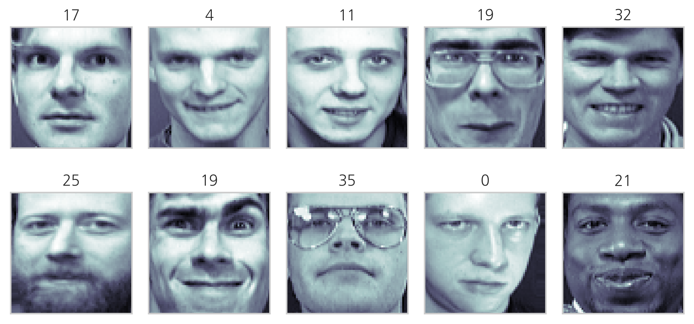
올리베티 얼굴 사진 데이터#
AT&T와 캠프리지 대학 전산 연구실에서 공동으로 제작한 얼굴 사진 데이터 베이스의 간략화된 버전. fetch_olivetti_faces() 명령으로 로드하며 다음과 같이 구성되어 있다. 64x64=4096 해상도의 흑백 이미지이고 40명의 사진 400장으로 구성되어 있다.
타겟 데이터
40명의 개인을 나타내는 식별 번호
특징 데이터
각 개인의 얼굴 이미지
from sklearn.datasets import fetch_olivetti_faces
olivetti = fetch_olivetti_faces()
print(olivetti.DESCR)
.. _olivetti_faces_dataset:

The Olivetti faces dataset
--------------------------

`This dataset contains a set of face images`_ taken between April 1992 and
April 1994 at AT&T Laboratories Cambridge. The
:func:`sklearn.datasets.fetch_olivetti_faces` function is the data
fetching / caching function that downloads the data
archive from AT&T.

.. _This dataset contains a set of face images: http://www.cl.cam.ac.uk/research/dtg/attarchive/facedatabase.html

As described on the original website:

    There are ten different images of each of 40 distinct subjects. For some
    subjects, the images were taken at different times, varying the lighting,
    facial expressions (open / closed eyes, smiling / not smiling) and facial
    details (glasses / no glasses). All the images were taken against a dark
    homogeneous background with the subjects in an upright, frontal position
    (with tolerance for some side movement).

**Data Set Characteristics:**

    =================   =====================
    Classes                                40
    Samples total                         400
    Dimensionality                       4096
    Features            real, between 0 and 1
    =================   =====================

The image is quantized to 256 grey levels and stored as unsigned 8-bit
integers; the loader will convert these to floating point values on the
interval [0, 1], which are easier to work with for many algorithms.

The "target" for this database is an integer from 0 to 39 indicating the
identity of the person pictured; however, with only 10 examples per class, this
relatively small dataset is more interesting from an unsupervised or
semi-supervised perspective.

The original dataset consisted of 92 x 112, while the version available here
consists of 64x64 images.

When using these images, please give credit to AT&T Laboratories Cambridge.
np.random.seed(0)
N = 2
M = 5
fig = plt.figure(figsize=(8, 5))
plt.subplots_adjust(top=1, bottom=0, hspace=0, wspace=0.05)
klist = np.random.choice(range(len(olivetti.data)), N * M)
for i in range(N):
    for j in range(M):
        k = klist[i*M+j]
        ax = fig.add_subplot(N, M, i*M+j+1)
        ax.imshow(olivetti.images[k], cmap=plt.cm.bone)
        ax.grid(False)
        ax.xaxis.set_ticks([])
        ax.yaxis.set_ticks([])
        plt.title(olivetti.target[k])
plt.tight_layout()
plt.show()
Labeled Faces in the Wild (LFW) 데이터#
유명 정치인 등의 실제 얼굴에 대한 이미지 데이터. fetch_lfw_people() 명령으로 로드한다. 해상도는 50x37=5,828픽셀이고 각 채널이 0~255의 정수값을 가지는 컬러 이미지이다. 5,749명의 13,233개 사진을 가지고 있다. 다음 인수를 사용하여 로드하는 데이터의 양과 종류를 결정할 수 있다.
funneled: 디폴트True이미지의 위치 조정(funnel) 여부
resize: 디폴트 0.5원래 이미지보다 일정 비율로 크기를 줄여서 로드
min_faces_per_person: 디폴트 None각 인물당 최소 사진의 수
color: 디폴트FalseTrue인 경우에는 컬러 사진을,False인 경우에는 흑백 사진을 로드한다.
from sklearn.datasets import fetch_lfw_people
lfw_people = fetch_lfw_people(min_faces_per_person=70, resize=0.4)
print(lfw_people.DESCR)
.. _labeled_faces_in_the_wild_dataset:

The Labeled Faces in the Wild face recognition dataset
------------------------------------------------------

This dataset is a collection of JPEG pictures of famous people collected
over the internet, all details are available on the official website:

    http://vis-www.cs.umass.edu/lfw/

Each picture is centered on a single face. The typical task is called
Face Verification: given a pair of two pictures, a binary classifier
must predict whether the two images are from the same person.

An alternative task, Face Recognition or Face Identification is:
given the picture of the face of an unknown person, identify the name
of the person by referring to a gallery of previously seen pictures of
identified persons.

Both Face Verification and Face Recognition are tasks that are typically
performed on the output of a model trained to perform Face Detection. The
most popular model for Face Detection is called Viola-Jones and is
implemented in the OpenCV library. The LFW faces were extracted by this
face detector from various online websites.

**Data Set Characteristics:**

    =================   =======================
    Classes                                5749
    Samples total                         13233
    Dimensionality                         5828
    Features            real, between 0 and 255
    =================   =======================

Usage
~~~~~

``scikit-learn`` provides two loaders that will automatically download,
cache, parse the metadata files, decode the jpeg and convert the
interesting slices into memmapped numpy arrays. This dataset size is more
than 200 MB. The first load typically takes more than a couple of minutes
to fully decode the relevant part of the JPEG files into numpy arrays. If
the dataset has  been loaded once, the following times the loading times
less than 200ms by using a memmapped version memoized on the disk in the
``~/scikit_learn_data/lfw_home/`` folder using ``joblib``.

The first loader is used for the Face Identification task: a multi-class
classification task (hence supervised learning)::

  >>> from sklearn.datasets import fetch_lfw_people
  >>> lfw_people = fetch_lfw_people(min_faces_per_person=70, resize=0.4)

  >>> for name in lfw_people.target_names:
  ...     print(name)
  ...
  Ariel Sharon
  Colin Powell
  Donald Rumsfeld
  George W Bush
  Gerhard Schroeder
  Hugo Chavez
  Tony Blair

The default slice is a rectangular shape around the face, removing
most of the background::

  >>> lfw_people.data.dtype
  dtype('float32')

  >>> lfw_people.data.shape
  (1288, 1850)

  >>> lfw_people.images.shape
  (1288, 50, 37)

Each of the ``1140`` faces is assigned to a single person id in the ``target``
array::

  >>> lfw_people.target.shape
  (1288,)

  >>> list(lfw_people.target[:10])
  [5, 6, 3, 1, 0, 1, 3, 4, 3, 0]

The second loader is typically used for the face verification task: each sample
is a pair of two picture belonging or not to the same person::

  >>> from sklearn.datasets import fetch_lfw_pairs
  >>> lfw_pairs_train = fetch_lfw_pairs(subset='train')

  >>> list(lfw_pairs_train.target_names)
  ['Different persons', 'Same person']

  >>> lfw_pairs_train.pairs.shape
  (2200, 2, 62, 47)

  >>> lfw_pairs_train.data.shape
  (2200, 5828)

  >>> lfw_pairs_train.target.shape
  (2200,)

Both for the :func:`sklearn.datasets.fetch_lfw_people` and
:func:`sklearn.datasets.fetch_lfw_pairs` function it is
possible to get an additional dimension with the RGB color channels by
passing ``color=True``, in that case the shape will be
``(2200, 2, 62, 47, 3)``.

The :func:`sklearn.datasets.fetch_lfw_pairs` datasets is subdivided into
3 subsets: the development ``train`` set, the development ``test`` set and
an evaluation ``10_folds`` set meant to compute performance metrics using a
10-folds cross validation scheme.

.. topic:: References:

 * `Labeled Faces in the Wild: A Database for Studying Face Recognition
   in Unconstrained Environments.
   <http://vis-www.cs.umass.edu/lfw/lfw.pdf>`_
   Gary B. Huang, Manu Ramesh, Tamara Berg, and Erik Learned-Miller.
   University of Massachusetts, Amherst, Technical Report 07-49, October, 2007.


Examples
~~~~~~~~

:ref:`sphx_glr_auto_examples_applications_plot_face_recognition.py`
np.random.seed(0)
N = 2
M = 5
fig = plt.figure(figsize=(8, 5))
plt.subplots_adjust(top=1, bottom=0, hspace=0.1, wspace=0.05)
klist = np.random.choice(range(len(lfw_people.data)), N * M)
for i in range(N):
    for j in range(M):
        k = klist[i*M+j]
        ax = fig.add_subplot(N, M, i*M+j+1)
        ax.imshow(lfw_people.images[k], cmap=plt.cm.bone)
        ax.grid(False)
        ax.xaxis.set_ticks([])
        ax.yaxis.set_ticks([])
        plt.title(lfw_people.target_names[lfw_people.target[k]])
plt.tight_layout()
plt.show()
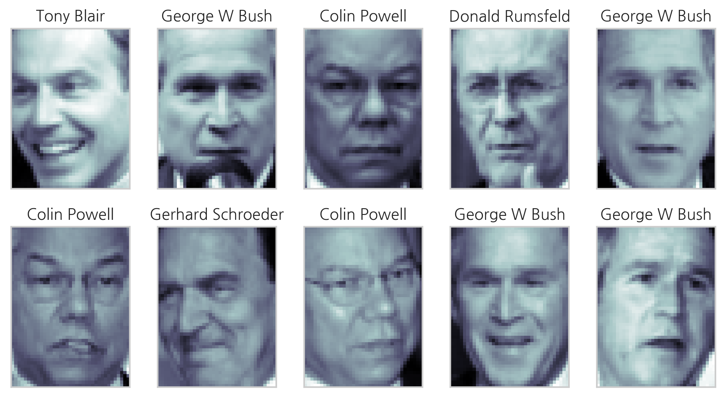
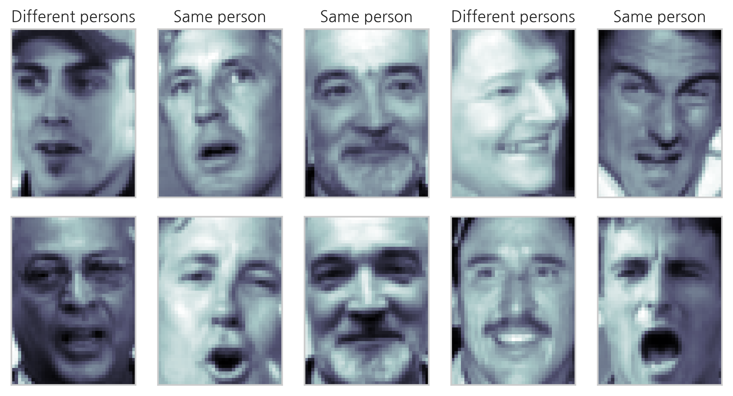
fetch_lfw_pairs() 명령을 사용하면 라벨이 아니라 한 쌍의 이미지 데이터를 로드하며 이 한 쌍의 사진은 동일 인물일 수도 있고 아닐 수도 있다. 타겟 데이터는 동일인인지 아닌지를 알려준다.
from sklearn.datasets import fetch_lfw_pairs
lfw_pairs = fetch_lfw_pairs(resize=0.4)
print(lfw_pairs.DESCR)
.. _labeled_faces_in_the_wild_dataset:

The Labeled Faces in the Wild face recognition dataset
------------------------------------------------------

This dataset is a collection of JPEG pictures of famous people collected
over the internet, all details are available on the official website:

    http://vis-www.cs.umass.edu/lfw/

Each picture is centered on a single face. The typical task is called
Face Verification: given a pair of two pictures, a binary classifier
must predict whether the two images are from the same person.

An alternative task, Face Recognition or Face Identification is:
given the picture of the face of an unknown person, identify the name
of the person by referring to a gallery of previously seen pictures of
identified persons.

Both Face Verification and Face Recognition are tasks that are typically
performed on the output of a model trained to perform Face Detection. The
most popular model for Face Detection is called Viola-Jones and is
implemented in the OpenCV library. The LFW faces were extracted by this
face detector from various online websites.

**Data Set Characteristics:**

    =================   =======================
    Classes                                5749
    Samples total                         13233
    Dimensionality                         5828
    Features            real, between 0 and 255
    =================   =======================

Usage
~~~~~

``scikit-learn`` provides two loaders that will automatically download,
cache, parse the metadata files, decode the jpeg and convert the
interesting slices into memmapped numpy arrays. This dataset size is more
than 200 MB. The first load typically takes more than a couple of minutes
to fully decode the relevant part of the JPEG files into numpy arrays. If
the dataset has  been loaded once, the following times the loading times
less than 200ms by using a memmapped version memoized on the disk in the
``~/scikit_learn_data/lfw_home/`` folder using ``joblib``.

The first loader is used for the Face Identification task: a multi-class
classification task (hence supervised learning)::

  >>> from sklearn.datasets import fetch_lfw_people
  >>> lfw_people = fetch_lfw_people(min_faces_per_person=70, resize=0.4)

  >>> for name in lfw_people.target_names:
  ...     print(name)
  ...
  Ariel Sharon
  Colin Powell
  Donald Rumsfeld
  George W Bush
  Gerhard Schroeder
  Hugo Chavez
  Tony Blair

The default slice is a rectangular shape around the face, removing
most of the background::

  >>> lfw_people.data.dtype
  dtype('float32')

  >>> lfw_people.data.shape
  (1288, 1850)

  >>> lfw_people.images.shape
  (1288, 50, 37)

Each of the ``1140`` faces is assigned to a single person id in the ``target``
array::

  >>> lfw_people.target.shape
  (1288,)

  >>> list(lfw_people.target[:10])
  [5, 6, 3, 1, 0, 1, 3, 4, 3, 0]

The second loader is typically used for the face verification task: each sample
is a pair of two picture belonging or not to the same person::

  >>> from sklearn.datasets import fetch_lfw_pairs
  >>> lfw_pairs_train = fetch_lfw_pairs(subset='train')

  >>> list(lfw_pairs_train.target_names)
  ['Different persons', 'Same person']

  >>> lfw_pairs_train.pairs.shape
  (2200, 2, 62, 47)

  >>> lfw_pairs_train.data.shape
  (2200, 5828)

  >>> lfw_pairs_train.target.shape
  (2200,)

Both for the :func:`sklearn.datasets.fetch_lfw_people` and
:func:`sklearn.datasets.fetch_lfw_pairs` function it is
possible to get an additional dimension with the RGB color channels by
passing ``color=True``, in that case the shape will be
``(2200, 2, 62, 47, 3)``.

The :func:`sklearn.datasets.fetch_lfw_pairs` datasets is subdivided into
3 subsets: the development ``train`` set, the development ``test`` set and
an evaluation ``10_folds`` set meant to compute performance metrics using a
10-folds cross validation scheme.

.. topic:: References:

 * `Labeled Faces in the Wild: A Database for Studying Face Recognition
   in Unconstrained Environments.
   <http://vis-www.cs.umass.edu/lfw/lfw.pdf>`_
   Gary B. Huang, Manu Ramesh, Tamara Berg, and Erik Learned-Miller.
   University of Massachusetts, Amherst, Technical Report 07-49, October, 2007.


Examples
~~~~~~~~

:ref:`sphx_glr_auto_examples_applications_plot_face_recognition.py`
np.random.seed(0)
N = 2
M = 5
fig = plt.figure(figsize=(8, 5))
plt.subplots_adjust(top=1, bottom=0, hspace=0.01, wspace=0.05)
klist = np.random.choice(range(len(lfw_pairs.data)), M)
for j in range(M):
    k = klist[j]
    ax1 = fig.add_subplot(N, M, j+1)
    ax1.imshow(lfw_pairs.pairs[k][0], cmap=plt.cm.bone)
    ax1.grid(False)
    ax1.xaxis.set_ticks([])
    ax1.yaxis.set_ticks([])
    plt.title(lfw_pairs.target_names[lfw_pairs.target[k]])
    ax2 = fig.add_subplot(N, M, j+1 + M)
    ax2.imshow(lfw_pairs.pairs[k][1], cmap=plt.cm.bone)
    ax2.grid(False)
    ax2.xaxis.set_ticks([])
    ax2.yaxis.set_ticks([])
plt.tight_layout()
plt.show()