6.1 로지스틱 회귀분석#
로지스틱(Logistic) 회귀분석은 회귀분석이라는 명칭과 달리 회귀분석 문제와 분류문제 모두에 사용할 수 있다. 로지스틱 회귀분석 모형에서는 종속변수가 이항분포를 따르고 그 모수 \(\mu\)가 독립변수 \(x\)에 의존한다고 가정한다.
위 식에서 보듯이 로지스틱 함수는 \(y\)의 값이 특정한 구간내의 값(\(0 \sim N\))만 가질 수 있기 때문에 종속변수가 이러한 특성을 가진 경우에 회귀분석 방법으로 쓸 수 있다.
또는 이항 분포의 특별한 경우(\(N=1\))로 \(y\)가 베르누이 확률분포인 경우도 있을 수 있다. 여기에서는 베르누이 확률분포를 따르는 로지스틱 회귀분석만 고려하기로 한다.
종속변수 \(y\)가 0또는 1인 분류 예측 문제를 풀 때는 \(x\) 값을 이용하여 \(\mu(x)\)를 예측한 후 다음 기준에 따라 \(\hat{y}\)값을 출력한다.
회귀분석을 할 때는 \(\hat{y}\)으로 \(y=1\)이 될 확률값 \(\mu(x)\)를 직접 사용한다.
시그모이드함수#
로지스틱 회귀모형에서는 베르누이 확률분포의 모수 \(\mu\)가 \(x\)의 함수라고 가정한다. \(\mu(x)\)는 \(x\)에 대한 함수를 0부터 1사이의 값만 나올 수 있도록 **시그모이드함수(sigmoid function)**라는 함수를 사용하여 변형한 것을 사용한다.
시그모이드함수는 종속변수의 모든 실수 값에 대해
유한한 구간 \((a,b)\) 사이의 한정된(bounded) 값을 가지고 $\( a < f(x) < b \)$
항상 양의 기울기를 가지는 단조증가하는 $\( a > b \; \rightarrow \; f(a) > f(b) \)$
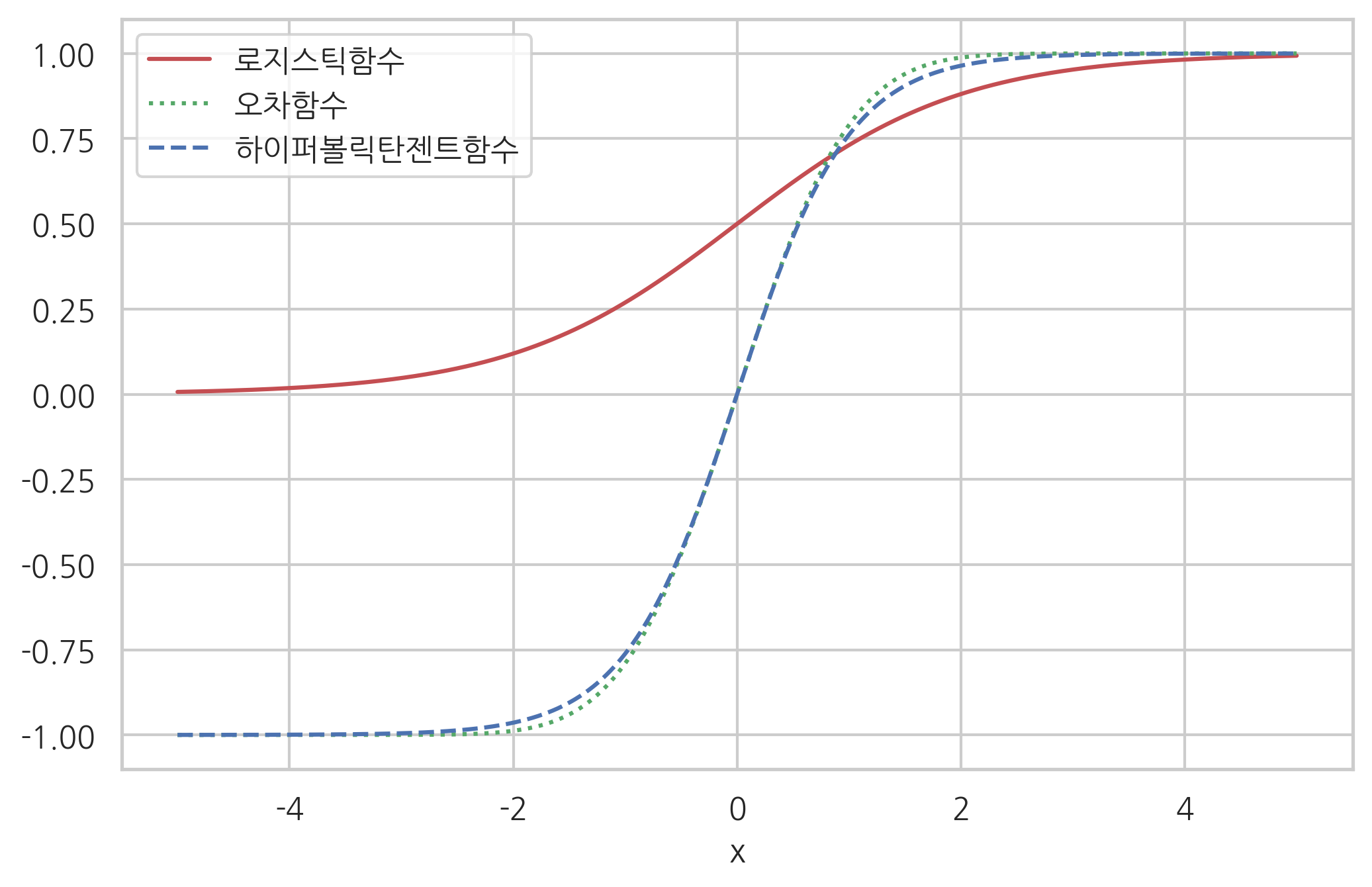
함수의 집합을 말한다. 실제로는 다음과 같은 함수들이 주로 사용된다.
로지스틱(Logistic)함수
하이퍼볼릭탄젠트(Hyperbolic tangent)함수
오차(Error)함수
하이퍼볼릭탄젠트함수는 로지스틱함수를 위아래 방향으로 2배 늘리고 좌우 방향으로 1/2로 축소한 것과 같다.
xx = np.linspace(-5, 5, 1000)
plt.plot(xx, 1/(1+np.exp(-xx)), 'r-', label="로지스틱함수")
plt.plot(xx, sp.special.erf(0.5*np.sqrt(np.pi)*xx), 'g:', label="오차함수")
plt.plot(xx, np.tanh(xx), 'b--', label="하이퍼볼릭탄젠트함수")
plt.ylim([-1.1, 1.1])
plt.legend(loc=2)
plt.xlabel("x")
plt.show()
로지스틱함수#
로지스틱함수는 음의 무한대부터 양의 무한대까지의 실수값을 0부터 1사이의 실수값으로 1 대 1 대응시키는 시그모이드함수다. 보통 시그모이드함수라고 하면 로지스틱함수를 가리킨다. 로지스틱함수는 다음 과정을 통해 정의되었다.
베르누이 시도에서 1이 나올 확률 \(\mu\)와 0이 나올 확률 \(1-\mu\)의 비율(ratio)을 승산비(odds ratio)라고 한다.
0부터 1사이의 값만 가지는 \(\mu\)를 승산비로 변환하면 0부터 양의 무한대까지의 값을 가질 수 있다.
승산비를 로그 변환한 것이 로지트함수(Logit function)다.
로지트함수의 값은 로그 변환에 의해 음의 무한대(\(-\infty\))부터 양의 무한대(\(\infty\))까지의 값을 가질 수 있다.
로지스틱함수(Logistic function)는 로지트함수의 역함수이다. 즉 음의 무한대(\(-\infty\))부터 양의 무한대(\(\infty\))까지의 값을 가지는 입력변수를 0부터 1사의 값을 가지는 출력변수로 변환한 것이다.
선형 판별함수#
로지스틱함수 \(\sigma(z)\)를 사용하는 경우에는 \(z\)값과 \(\mu\)값은 다음과 같은 관계가 있다.
\(z = 0\)일 때 \(\mu = 0.5\)
\(z > 0\)일 때 \(\mu > 0.5 \; \rightarrow \hat{y} = 1\)
\(z < 0\)일 때 \(\mu < 0.5 \; \rightarrow \hat{y} = 0\)
즉 \(z\)가 분류 모형의 판별함수(decision function)의 역할을 한다. 로지스틱 회귀분석에서는 판별함수 수식으로 선형함수를 사용한다.
따라서 판별 경계면도 선형이 된다.
로지스틱 회귀분석 모형의 모수 추정#
로지스틱 회귀분석 모형의 모수 \(w\)는 최대가능도(Maximum Likelihood Estimation, MLE)방법으로 추정할 수 있다.
우선 베르누이분포의 확률밀도함수는 다음과 같다.
\(\mu\)는 \(w^Tx\)에 로지스틱함수를 적용한 값이다.
이 식을 대입하면 조건부 확률은 다음과 같다.
데이터 표본이 \(\{ x_i, y_i \}_{1:N}\)로 여러 개 있는 경우 전체 데이터의 로그가능도 \({LL}\)를 구하면 다음과 같다.
베르누이 확률분포의 정의에서
가 된다.
로그가능도를 최대화하는 \(w\) 값을 구하기 위해 모수로 미분한다.
\(LL\)을 \(\mu\)로 미분하면
\(\mu\)를 \(w\)로 미분하면
두 식을 곱하면 그레디언트 벡터의 수식을 구할 수 있다.
그레디언트 벡터가 영벡터가 되는 모수의 값이 로그가능도를 최대화하는 값이다. 하지만 그레디언트 벡터 수식이 \(w\)에 대한 비선형 함수이므로 선형 모형과 같이 간단하게 그레디언트가 0이 되는 모수 \(w\) 값에 대한 수식을 구할 수 없으며 수치적인 최적화 방법(numerical optimization)을 통해 반복적으로 최적 모수 \(w\)의 값을 구해야 한다.
수치적 최적화#
로그가능도함수 \(LL\)을 최대화하는 것은 다음 목적함수를 최소화하는 것과 같다.
최대경사도(Steepest Gradient Descent)방법을 사용하자.
그레디언트 벡터는 $\( g_k = \dfrac{d}{dw}(-LL) \)$
이고, 이 방향으로 스텝사이즈 \(\eta_k\)만큼 이동한다.
StatsModels 패키지의 로지스틱 회귀#
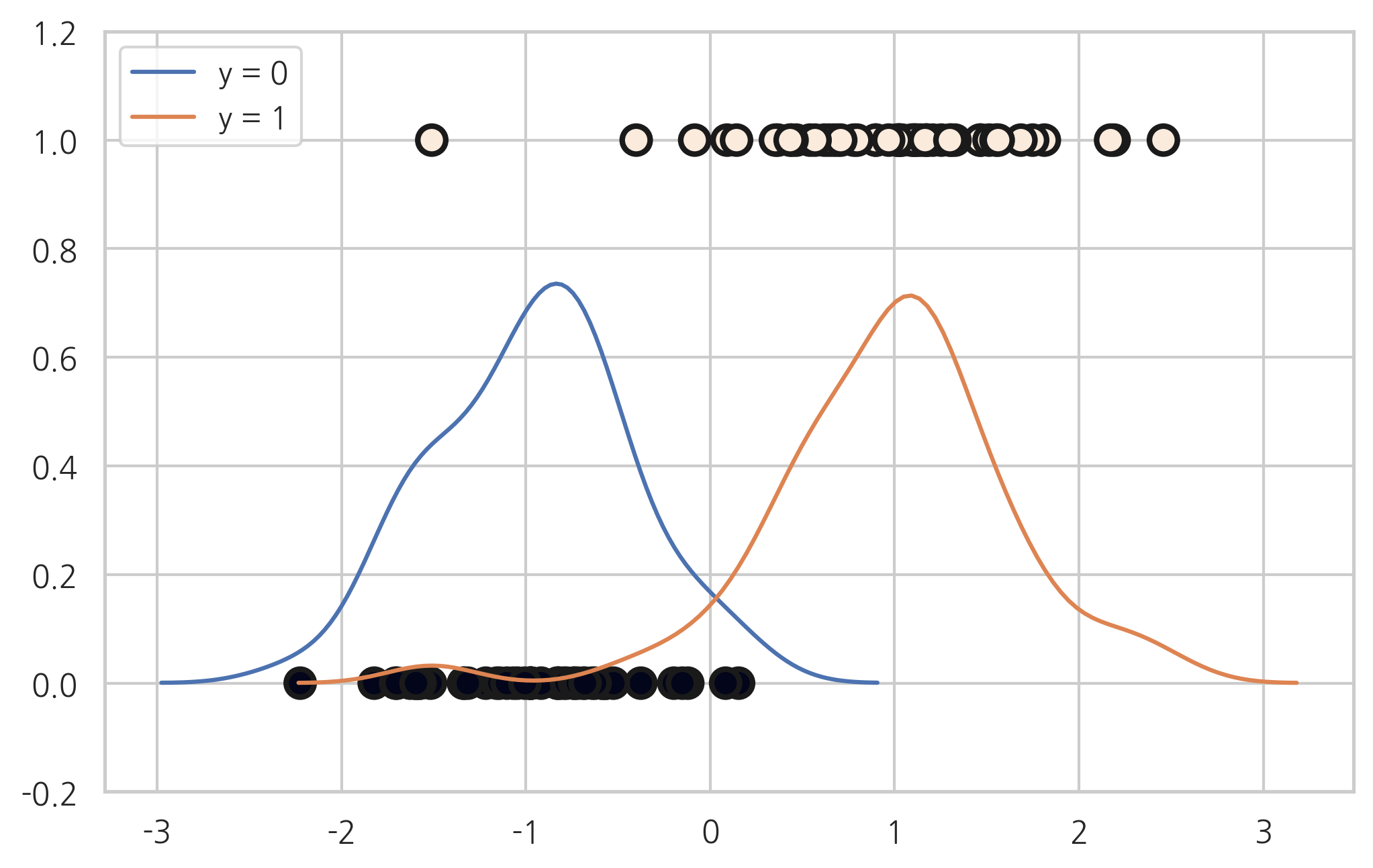
다음과 같은 1차원 독립변수를 가지는 분류문제를 풀어보자.
from sklearn.datasets import make_classification

X0, y = make_classification(n_features=1, n_redundant=0, n_informative=1,
                            n_clusters_per_class=1, random_state=4)

plt.scatter(X0, y, c=y, s=100, edgecolor="k", linewidth=2)
sns.distplot(X0[y == 0, :], label="y = 0", hist=False)
sns.distplot(X0[y == 1, :], label="y = 1", hist=False)
plt.ylim(-0.2, 1.2)
plt.show()
StatsModels 패키지는 베르누이 분포를 따르는 로지스틱 회귀 모형 Logit 를 제공한다. 사용방법은 OLS 클래스 사용법과 동일하다. 종속변수와 독립변수 데이터를 넣어 모형을 만들고 fit 메서드로 학습을 시킨다. fit 메서드의 disp=0 인수는 최적화 과정에서 문자열 메세지를 나타내지 않는 역할을 한다.
X = sm.add_constant(X0)
logit_mod = sm.Logit(y, X)
logit_res = logit_mod.fit(disp=0)
print(logit_res.summary())
                           Logit Regression Results
==============================================================================
Dep. Variable:                      y   No. Observations:                  100
Model:                          Logit   Df Residuals:                       98
Method:                           MLE   Df Model:                            1
Date:                Sat, 06 Jun 2020   Pseudo R-squ.:                  0.7679
Time:                        10:01:05   Log-Likelihood:                -16.084
converged:                       True   LL-Null:                       -69.295
Covariance Type:            nonrobust   LLR p-value:                 5.963e-25
==============================================================================
                 coef    std err          z      P>|z|      [0.025      0.975]
------------------------------------------------------------------------------
const          0.2515      0.477      0.527      0.598      -0.683       1.186
x1             4.2382      0.902      4.699      0.000       2.470       6.006
==============================================================================
결과 객체에서 summary 메서드를 사용하여 리포트를 출력할 수 있다. 결과 리포트에서 판별함수의 수식이 다음과 같다는 것을 알 수 있다.
따라서 \(z\)값의 부호를 나누는 기준값은 \(4.2382x + 0.2515 = 0.5\)가 되는 \(x\)값 즉, \((0.5-0.2515)/4.2382\)다.
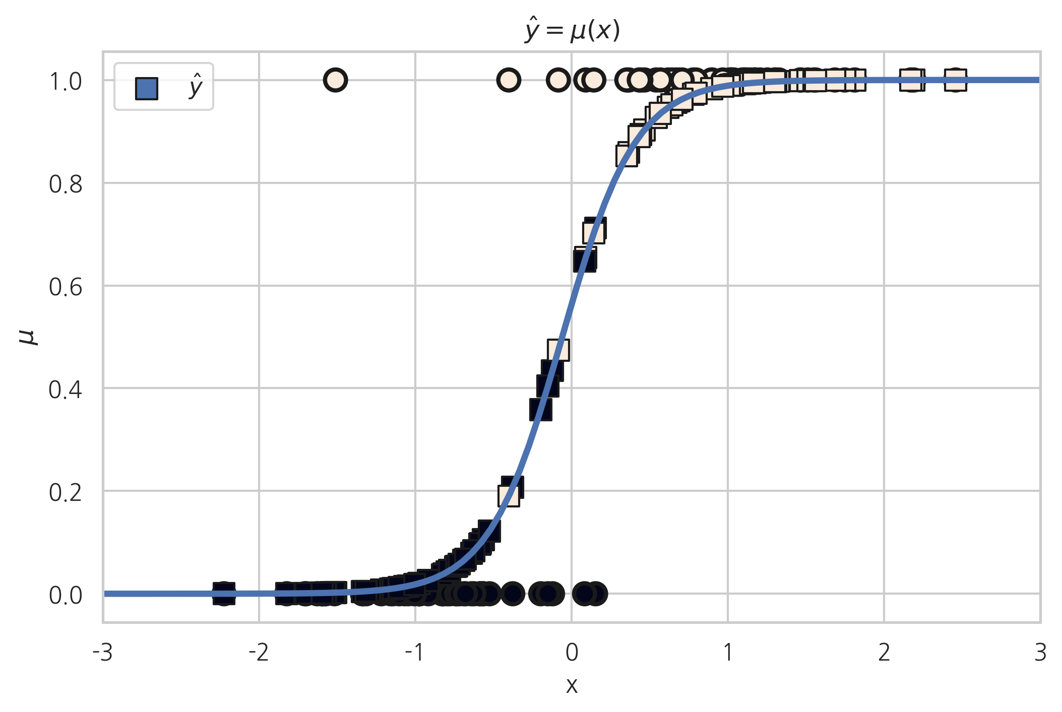
predict 메서드를 사용하면 \(\mu(x)\)값을 출력한다.
유의확률을 감안하면 상수항의 값은 0과 마찬가지이므로 \(\mu(x)\)가 다음과 같다고 볼 수도 있다.
이렇게 생각하면 \(z\)값의 부호를 나누는 기준값은 실질적으로는 \(0.5/4.2382=0.118\)이다.
xx = np.linspace(-3, 3, 100)
mu = logit_res.predict(sm.add_constant(xx))
plt.plot(xx, mu, lw=3)
plt.scatter(X0, y, c=y, s=100, edgecolor="k", lw=2)
plt.scatter(X0, logit_res.predict(X), label=r"$\hat{y}$", marker='s', c=y,
            s=100, edgecolor="k", lw=1)
plt.xlim(-3, 3)
plt.xlabel("x")
plt.ylabel(r"$\mu$")
plt.title(r"$\hat{y} = \mu(x)$")
plt.legend()
plt.show()
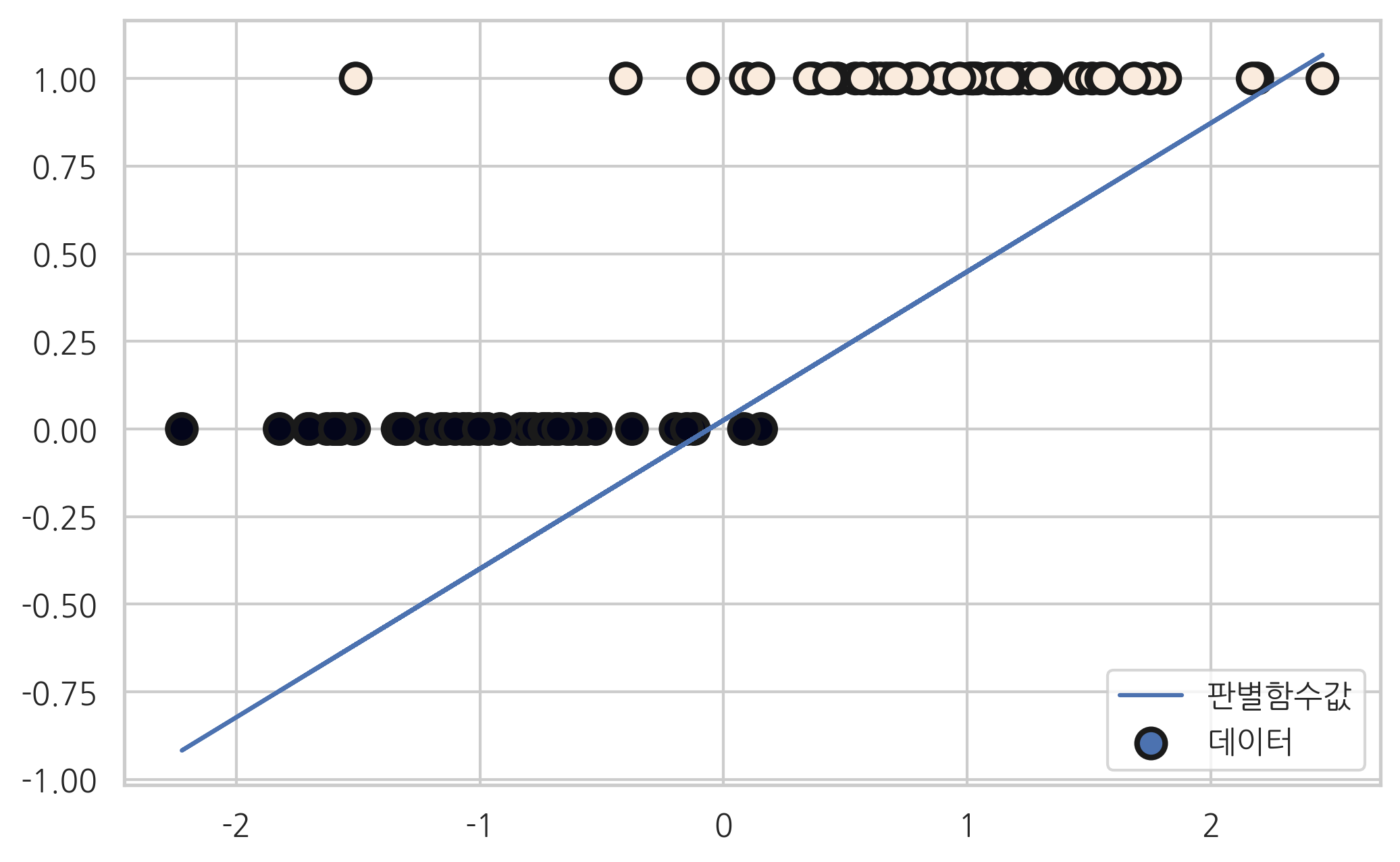
판별함수#
Logit 모형의 결과 객체에는 fittedvalues라는 속성으로 판별함수 \(z=w^Tx\) 값이 들어가 있다. 이 값을 이용하여 분류문제를 풀 수도 있다.
plt.scatter(X0, y, c=y, s=100, edgecolor="k", lw=2, label="데이터")
plt.plot(X0, logit_res.fittedvalues * 0.1, label="판별함수값")
plt.legend()
plt.show()
로지스틱 회귀 성능 측정#
로지스틱 회귀 성능은 맥파든 의사결정계수(McFadden pseudo R square)값으로 측정한다.
\(G^2\)는 이탈도(deviance)라고 하는 양으로 다음과 같이 정의된다.
여기에서 \(\hat{y}\)는 \(y=1\)일 확률 \(\mu\)를 뜻한다.
이탈도는 모형이 100% 정확한 경우에는 0이 되고 모형의 성능이 나빠질수록 값이 커진다.
또한 이탈도는 로그 가능도에 음수를 취한 값과 같다.
\(G^2\)는 현재 이탈도이고 \(G^2_0\)는 귀무모형(null model)으로 측정한 이탈도다.
귀무모형이란 모든 \(x\)가 \(y\)를 예측하는데 전혀 영향을 미치지 않는 모형을 말한다. 즉, 무조건부 확률 \(p(y)\)에 따라 \(x\)에 상관없이 동일하게 \(y\)를 예측하는 모형을 말한다. 결국 우리가 만들 수 있는 가장 성능이 나쁜 모형이 된다.
따라서 맥파든 의사결정계수는 가장 성능이 좋을 때는 1이 되고 가장 성능이 나쁠 때는 0이 된다.
scikit-learn 패키지의 metric 서브패키지에는 로그 손실을 계산하는 log_loss 함수가 있다. normalize=False로 놓으면 이탈도와 같은 값을 구한다
위 예제에서 최적 모형의 로그 손실은 약 16.08로 계산된다.
from sklearn.metrics import log_loss

y_hat = logit_res.predict(X)
log_loss(y, y_hat, normalize=False)
16.084355200413036
귀무 모형의 모수값을 구하면 0.51이고 이 값으로 로그 손실을 계산하면 약 69이다.
mu_null = np.sum(y) / len(y)
mu_null
0.51
y_null = np.ones_like(y) * mu_null
log_loss(y, y_null, normalize=False)
69.29471672244784
두 값을 이용하여 맥파든 의사 결정계수 값을 계산할 수 있다.
1 - (log_loss(y, y_hat) / log_loss(y, y_null))
0.7678848264170398
Scikit-Learn 패키지의 로지스틱 회귀#
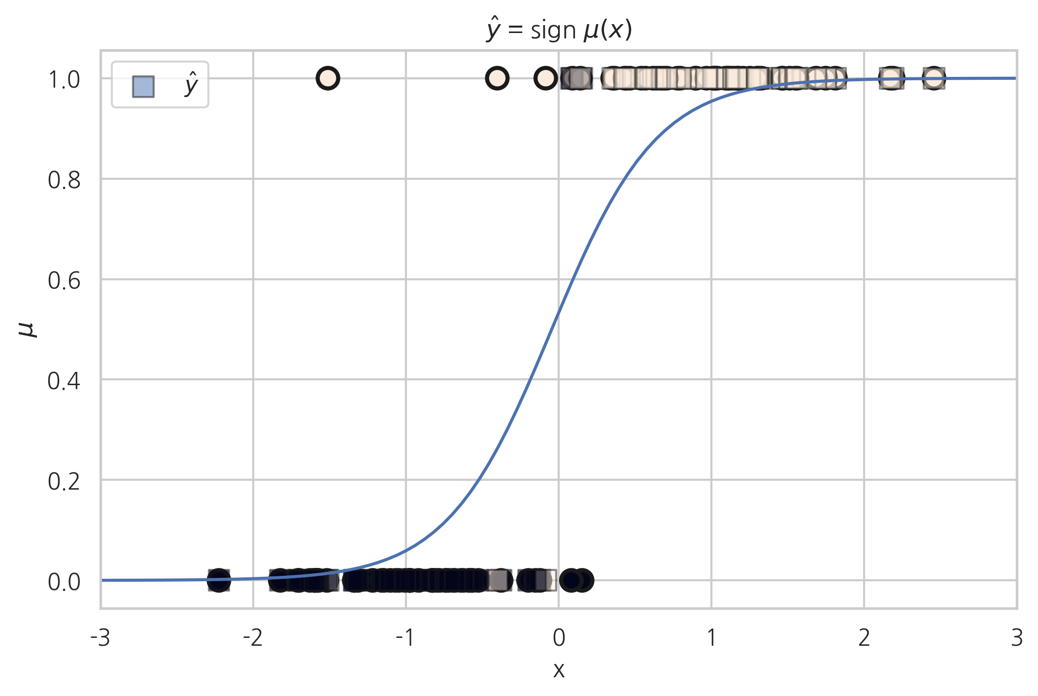
Scikit-Learn 패키지는 로지스틱 회귀 모형 LogisticRegression 를 제공한다.
from sklearn.linear_model import LogisticRegression

model_sk = LogisticRegression().fit(X0, y)

xx = np.linspace(-3, 3, 100)
mu = 1.0/(1 + np.exp(-model_sk.coef_[0][0]*xx - model_sk.intercept_[0]))
plt.plot(xx, mu)
plt.scatter(X0, y, c=y, s=100, edgecolor="k", lw=2)
plt.scatter(X0, model_sk.predict(X0), label=r"$\hat{y}$", marker='s', c=y,
            s=100, edgecolor="k", lw=1, alpha=0.5)
plt.xlim(-3, 3)
plt.xlabel("x")
plt.ylabel(r"$\mu$")
plt.title(r"$\hat{y}$ = sign $\mu(x)$")
plt.legend()
plt.show()
연습 문제 1#
붓꽃 분류문제에서 클래스가 세토사와 베르시칼라 데이터만 사용하고 (setosa=0, versicolor=1) 독립변수로는 꽃받침 길이(Sepal Length)와 상수항만 사용하여 StatsModels 패키지의 로지스틱 회귀모형으로 결과를 예측하고 보고서를 출력한다. 이 보고서에서 어떤 값이 세토사와 베르시칼라를 구분하는 기준값(threshold)으로 사용되고 있는가?
위 결과를 분류결과표(confusion matrix)와 분류결과보고서(classification report)로 나타내라.
이 모형에 대해 ROC커브를 그리고 AUC를 구한다. 이 때 Scikit-Learn의
LogisticRegression을 사용하지 않고 위에서 StatsModels로 구한 모형을 사용한다.
from sklearn.datasets import load_iris

iris = load_iris()
X = iris.data
y = iris.target
dfX = pd.DataFrame(X, columns=iris.feature_names)
dfy = pd.DataFrame(y, columns=["species"])
df = pd.concat([dfX, dfy], axis=1)
df = df[["sepal length (cm)", "species"]]
df = df[df.species.isin([0, 1])]
df = df.rename(columns={"sepal length (cm)": "sepal_length" })

import statsmodels.api as sm

model = sm.Logit.from_formula("species ~ sepal_length", data=df)
result = model.fit()
print(result.summary())
Optimization terminated successfully.
         Current function value: 0.321056
         Iterations 8
                           Logit Regression Results
==============================================================================
Dep. Variable:                species   No. Observations:                  100
Model:                          Logit   Df Residuals:                       98
Method:                           MLE   Df Model:                            1
Date:                Sat, 06 Jun 2020   Pseudo R-squ.:                  0.5368
Time:                        10:01:22   Log-Likelihood:                -32.106
converged:                       True   LL-Null:                       -69.315
Covariance Type:            nonrobust   LLR p-value:                 6.320e-18
================================================================================
                   coef    std err          z      P>|z|      [0.025      0.975]
--------------------------------------------------------------------------------
Intercept      -27.8315      5.434     -5.122      0.000     -38.481     -17.182
sepal_length     5.1403      1.007      5.107      0.000       3.168       7.113
================================================================================
# 기준값
(0.5 + 27.8315) /  5.1403
5.511643289302181
y_pred = result.predict(df.sepal_length) >= 0.5

from sklearn.metrics import confusion_matrix

confusion_matrix(df.species, y_pred)
array([[45,  5],
       [ 6, 44]])
from sklearn.metrics import classification_report

print(classification_report(df.species, y_pred))
              precision    recall  f1-score   support

           0       0.88      0.90      0.89        50
           1       0.90      0.88      0.89        50

    accuracy                           0.89       100
   macro avg       0.89      0.89      0.89       100
weighted avg       0.89      0.89      0.89       100
from sklearn.metrics import roc_curve

fpr, tpr, thresholds = roc_curve(df.species, result.predict(df.sepal_length))
plt.plot(fpr, tpr)
plt.show()
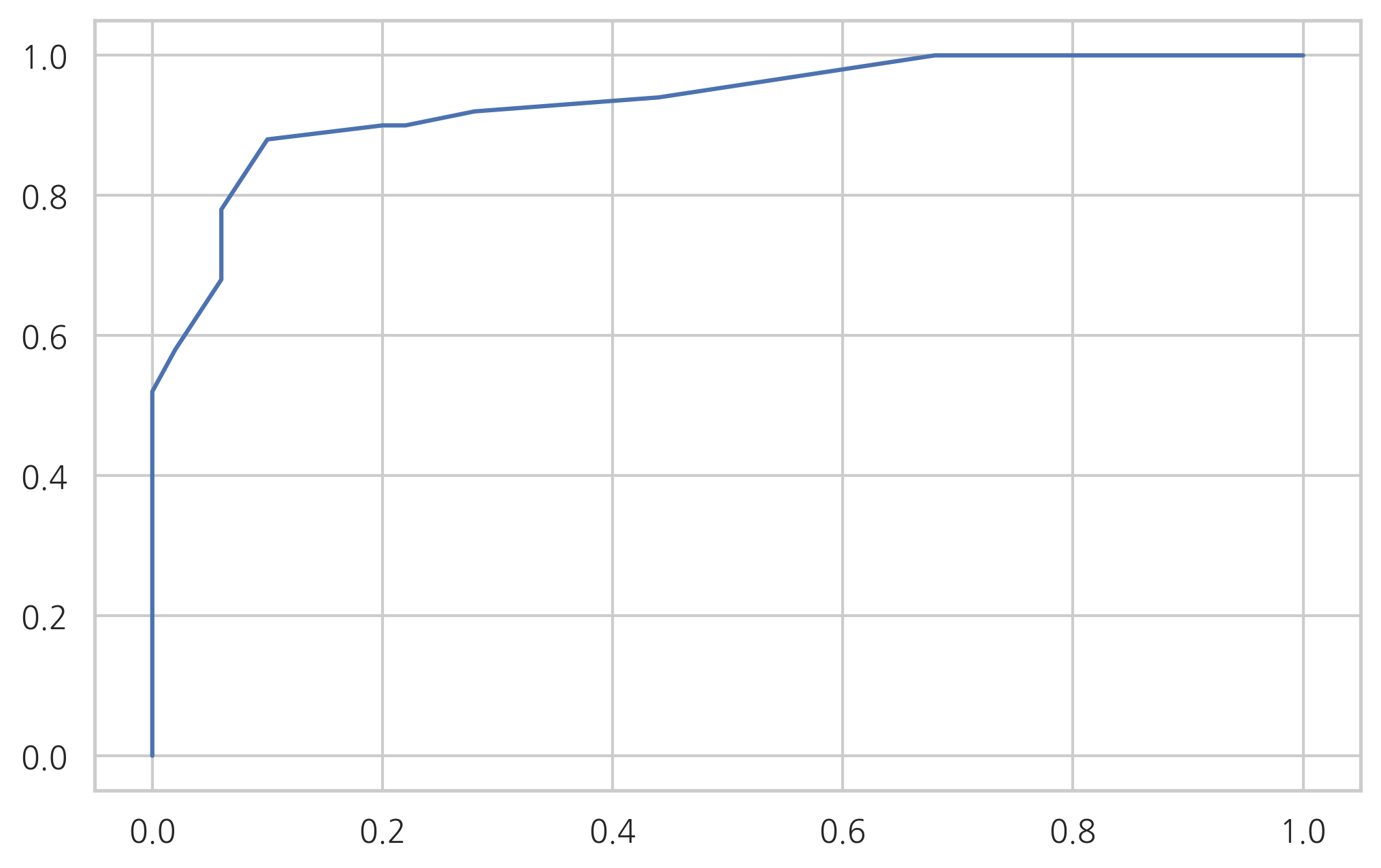
from sklearn.metrics import auc
auc(fpr, tpr)
0.9326
로지스틱 회귀를 사용한 이진 분류의 예#
다음 데이터는 미국 의대생의 입학관련 데이터이다. 데이터의 의미는 다음과 같다.
Acceptance: 0이면 불합격, 1이면 합격BCPM: Bio/Chem/Physics/Math 과목의 학점 평균GPA: 전체과목 학점 평균VR: MCAT Verbal reasoning 과목 점수PS: MCAT Physical sciences 과목 점수WS: MCAT Writing sample 과목 점수BS: MCAT Biological sciences 과목 점수MCAT: MCAT 촘점Apps: 의대 지원 횟수
data_med = sm.datasets.get_rdataset("MedGPA", package="Stat2Data")
df_med = data_med.data
df_med.tail()
| Accept | Acceptance | Sex | BCPM | GPA | VR | PS | WS | BS | MCAT | Apps | |
|---|---|---|---|---|---|---|---|---|---|---|---|
| 50 | D | 0 | M | 2.41 | 2.72 | 8 | 8 | 8.0 | 8 | 32 | 7 |
| 51 | D | 0 | M | 3.51 | 3.56 | 11 | 8 | 6.0 | 9 | 34 | 6 |
| 52 | A | 1 | F | 3.43 | 3.48 | 7 | 10 | 7.0 | 10 | 34 | 14 |
| 53 | D | 0 | M | 2.61 | 2.80 | 7 | 5 | NaN | 6 | 18 | 6 |
| 54 | D | 0 | M | 3.36 | 3.44 | 11 | 11 | 8.0 | 9 | 39 | 1 |
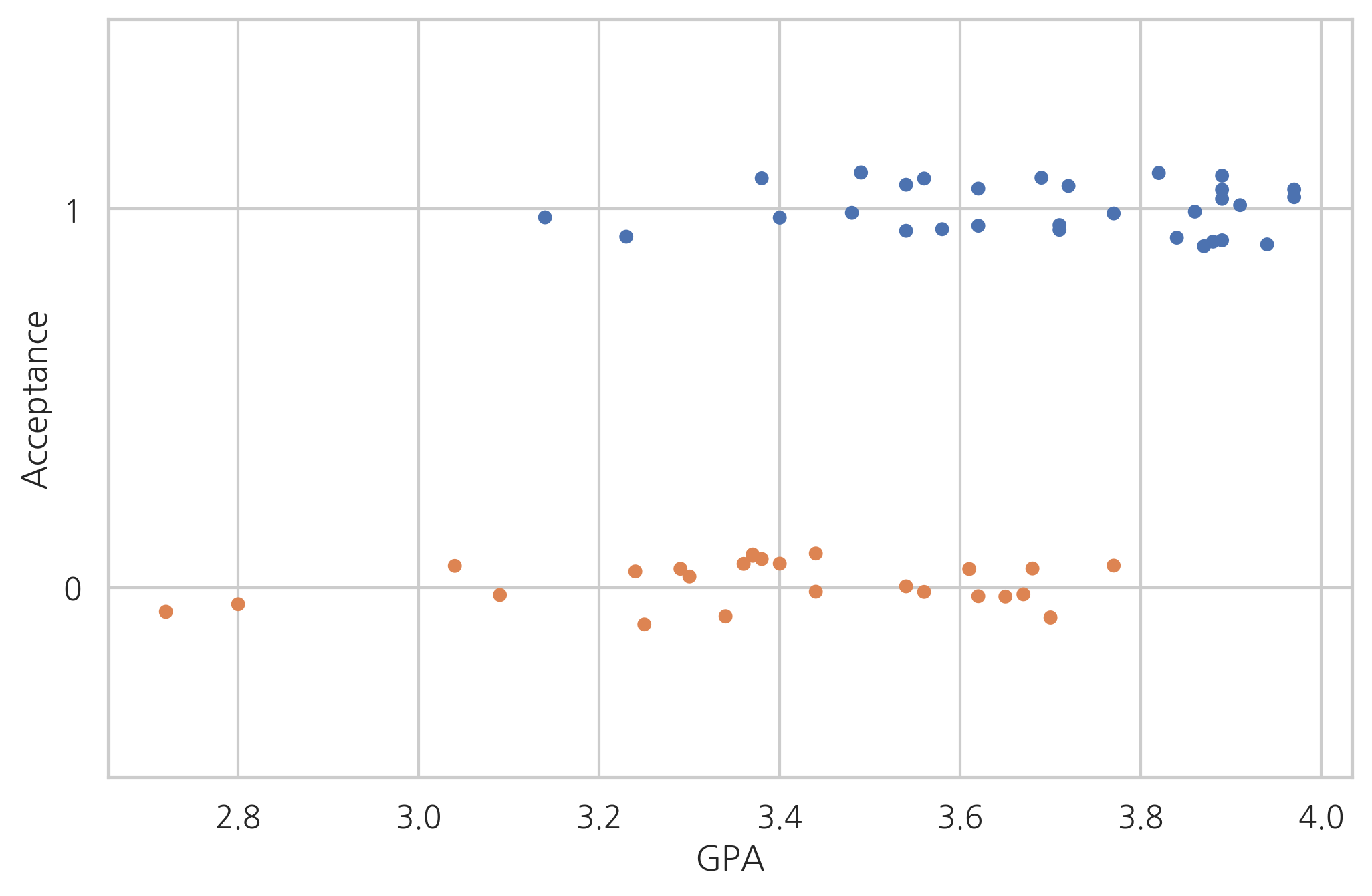
일단 학점(GPA)과 합격여부의 관계를 살펴보자.
sns.stripplot(x="GPA", y="Acceptance", data=df_med,
              jitter=True, orient='h', order=[1, 0])
plt.grid(True)
plt.show()
로지스틱 회귀분석을 실시한다. MCAT = VR + PS + WS + BS이므로 이 MCAT은 독립 변수에서 제외해야 한다.
model_med = sm.Logit.from_formula("Acceptance ~ Sex + BCPM + GPA + VR + PS + WS + BS + Apps", df_med)
result_med = model_med.fit()
print(result_med.summary())
Optimization terminated successfully.
         Current function value: 0.280736
         Iterations 9
                           Logit Regression Results
==============================================================================
Dep. Variable:             Acceptance   No. Observations:                   54
Model:                          Logit   Df Residuals:                       45
Method:                           MLE   Df Model:                            8
Date:                Sat, 06 Jun 2020   Pseudo R-squ.:                  0.5913
Time:                        10:01:33   Log-Likelihood:                -15.160
converged:                       True   LL-Null:                       -37.096
Covariance Type:            nonrobust   LLR p-value:                 6.014e-07
==============================================================================
                 coef    std err          z      P>|z|      [0.025      0.975]
------------------------------------------------------------------------------
Intercept    -46.6414     15.600     -2.990      0.003     -77.216     -16.067
Sex[T.M]      -2.2835      1.429     -1.597      0.110      -5.085       0.518
BCPM          -6.1633      6.963     -0.885      0.376     -19.811       7.484
GPA           12.3973      8.611      1.440      0.150      -4.479      29.274
VR             0.0790      0.311      0.254      0.799      -0.530       0.688
PS             1.1673      0.539      2.164      0.030       0.110       2.225
WS            -0.7784      0.396     -1.968      0.049      -1.554      -0.003
BS             1.9184      0.682      2.814      0.005       0.582       3.255
Apps           0.0512      0.147      0.348      0.728      -0.237       0.340
==============================================================================
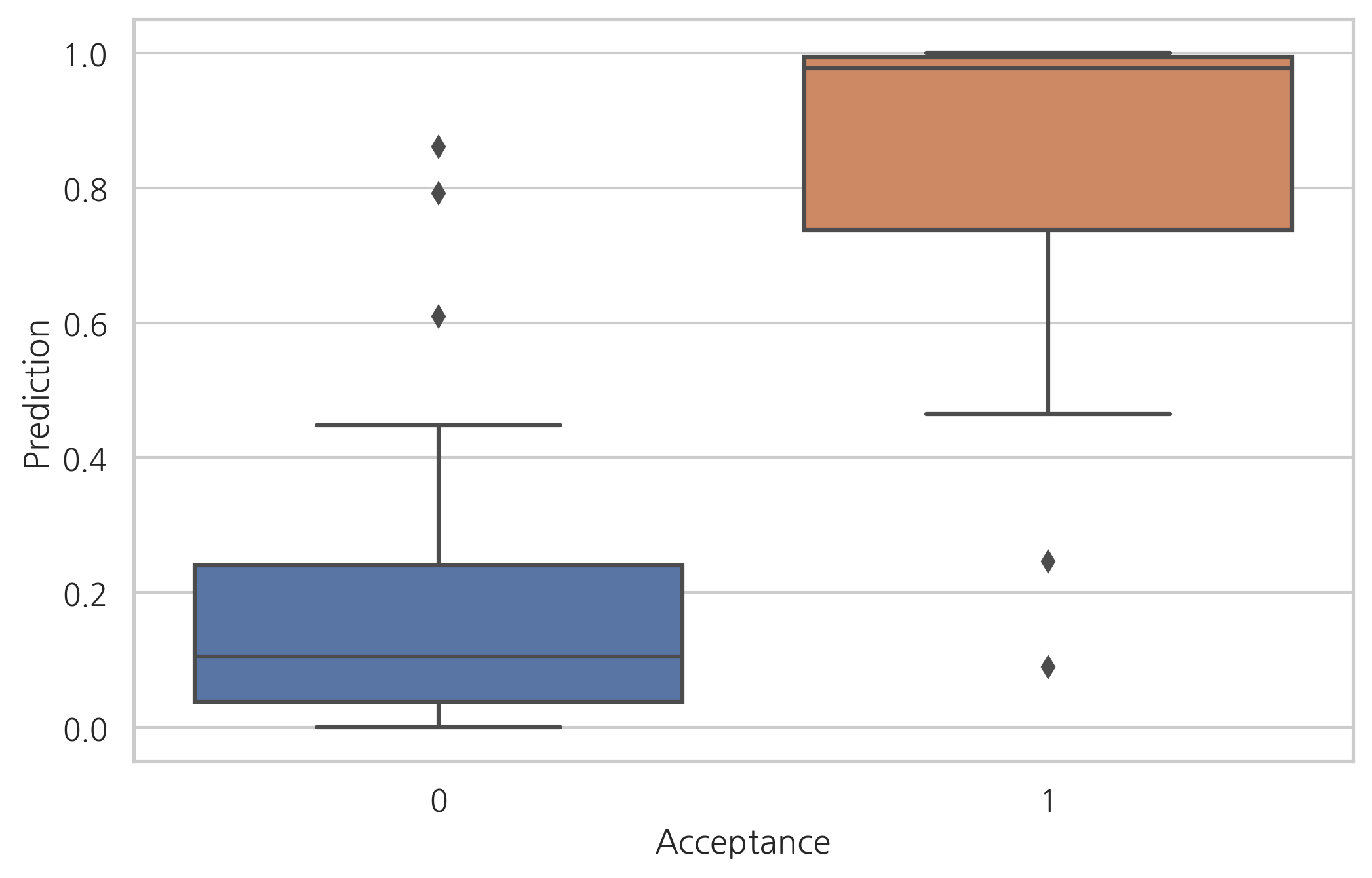
예측 결과와 실제 결과를 비교하면 다음과 같다.
df_med["Prediction"] = result_med.predict(df_med)
sns.boxplot(x="Acceptance", y="Prediction", data=df_med)
plt.show()
위 분석 결과를 토대로 유의하지 않은 변수들을 제외하고 PS와 BS 점수만을 이용하여 다시 회귀분석하면 다음과 같다.
model_med = sm.Logit.from_formula("Acceptance ~ PS + BS", df_med)
result_med = model_med.fit()
print(result_med.summary())
Optimization terminated successfully.
         Current function value: 0.460609
         Iterations 7
                           Logit Regression Results
==============================================================================
Dep. Variable:             Acceptance   No. Observations:                   55
Model:                          Logit   Df Residuals:                       52
Method:                           MLE   Df Model:                            2
Date:                Sat, 06 Jun 2020   Pseudo R-squ.:                  0.3315
Time:                        10:01:36   Log-Likelihood:                -25.333
converged:                       True   LL-Null:                       -37.896
Covariance Type:            nonrobust   LLR p-value:                 3.503e-06
==============================================================================
                 coef    std err          z      P>|z|      [0.025      0.975]
------------------------------------------------------------------------------
Intercept    -15.5427      4.684     -3.318      0.001     -24.723      -6.362
PS             0.4798      0.316      1.518      0.129      -0.140       1.099
BS             1.1464      0.387      2.959      0.003       0.387       1.906
==============================================================================
위 결과를 바탕으로 다음 점수가 \(15.5427+0.5\)보다 크면 합격이라고 예측할 수 있다.
연습 문제 2#
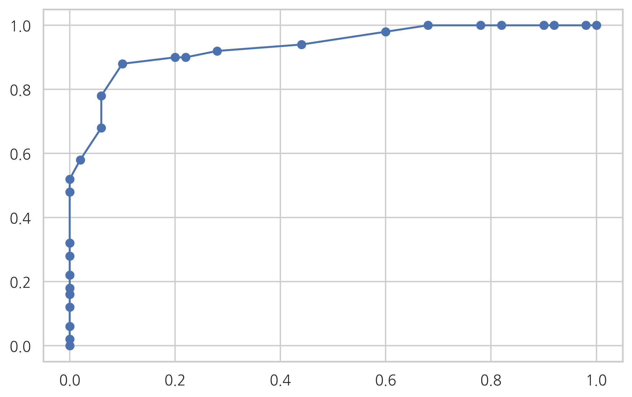
붓꽃 분류문제에서 클래스가 베르시칼라(versicolor)와 버지니카(virginica) 데이터만 사용하여(versicolor=1, virginica=2) 로지스틱 회귀모형으로 결과를 예측하고 보고서를 출력한다. 독립변수는 모두 사용한다. 이 보고서에서 버지니카와 베르시칼라를 구분하는 경계면의 방정식을 찾아라.
위 결과를 분류결과표와 분류결과보고서로 나타내라.
이 모형에 대해 ROC커브를 그리고 AUC를 구하라. 이 때 Scikit-Learn의
LogisticRegression을 사용하지 않고 위에서 StatsModels로 구한 모형을 사용한다.
from sklearn.datasets import load_iris

iris = load_iris()
X = iris.data
y = iris.target
dfX = pd.DataFrame(X, columns=iris.feature_names)
dfy = pd.DataFrame(y, columns=["species"])
df = pd.concat([dfX, dfy], axis=1)
df = df[df.species.isin([1, 2])]
df["species"] -= 1
df = df.rename(
    columns={
        "sepal length (cm)": "sepal_length",
        "sepal width (cm)": "sepal_width",
        "petal length (cm)": "petal_length",
        "petal width (cm)": "petal_width",
    }
)

import statsmodels.api as sm

model = sm.Logit.from_formula(
    "species ~ sepal_length + sepal_width + petal_length + petal_width",
    data=df)
result = model.fit()
print(result.summary())
Optimization terminated successfully.
         Current function value: 0.059493
         Iterations 12
                           Logit Regression Results
==============================================================================
Dep. Variable:                species   No. Observations:                  100
Model:                          Logit   Df Residuals:                       95
Method:                           MLE   Df Model:                            4
Date:                Sat, 06 Jun 2020   Pseudo R-squ.:                  0.9142
Time:                        10:01:37   Log-Likelihood:                -5.9493
converged:                       True   LL-Null:                       -69.315
Covariance Type:            nonrobust   LLR p-value:                 1.947e-26
================================================================================
                   coef    std err          z      P>|z|      [0.025      0.975]
--------------------------------------------------------------------------------
Intercept      -42.6378     25.708     -1.659      0.097     -93.024       7.748
sepal_length    -2.4652      2.394     -1.030      0.303      -7.158       2.228
sepal_width     -6.6809      4.480     -1.491      0.136     -15.461       2.099
petal_length     9.4294      4.737      1.990      0.047       0.145      18.714
petal_width     18.2861      9.743      1.877      0.061      -0.809      37.381
================================================================================

Possibly complete quasi-separation: A fraction 0.60 of observations can be
perfectly predicted. This might indicate that there is complete
quasi-separation. In this case some parameters will not be identified.
y_pred = result.predict(df) >= 0.5

from sklearn.metrics import confusion_matrix

confusion_matrix(df.species, y_pred)
array([[49,  1],
       [ 1, 49]])
from sklearn.metrics import classification_report

print(classification_report(df.species, y_pred))
              precision    recall  f1-score   support

           0       0.98      0.98      0.98        50
           1       0.98      0.98      0.98        50

    accuracy                           0.98       100
   macro avg       0.98      0.98      0.98       100
weighted avg       0.98      0.98      0.98       100
from sklearn.metrics import roc_curve

fpr, tpr, thresholds = roc_curve(df.species, result.predict(df))
plt.plot(fpr, tpr)
plt.show()
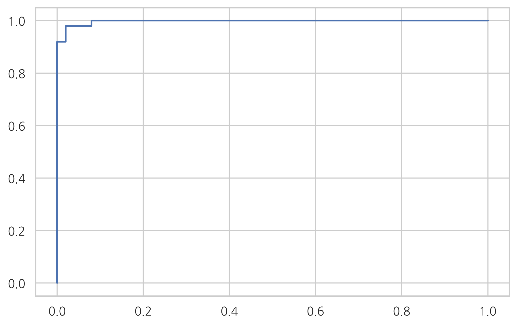
from sklearn.metrics import auc
auc(fpr, tpr)
0.9972000000000001
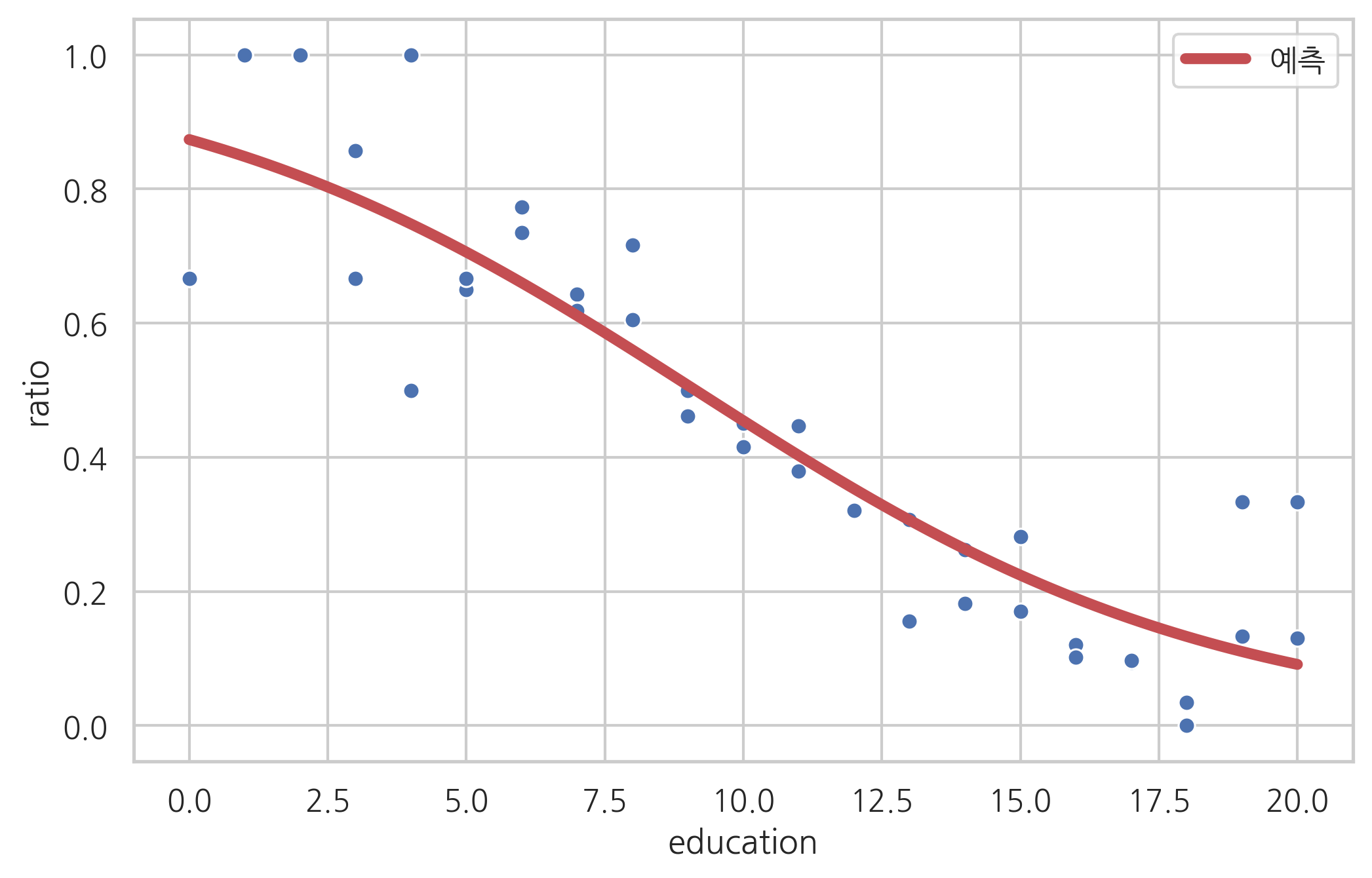
로지스틱 회귀를 사용한 회귀분석#
로지스틱 회귀는 분류문제뿐만 아니라 종속변수 \(y\)가 0부터 1까지 막혀있는 회귀분석 문제에도 사용할 수 있다. 이때는 다음처럼 \(\mu\) 값을 종속변수 y의 예측값으로 사용한다.
만약 실제 y의 범위가 0부터 1이 아니면 스케일링을 통해 바꿔야 한다.
예제#
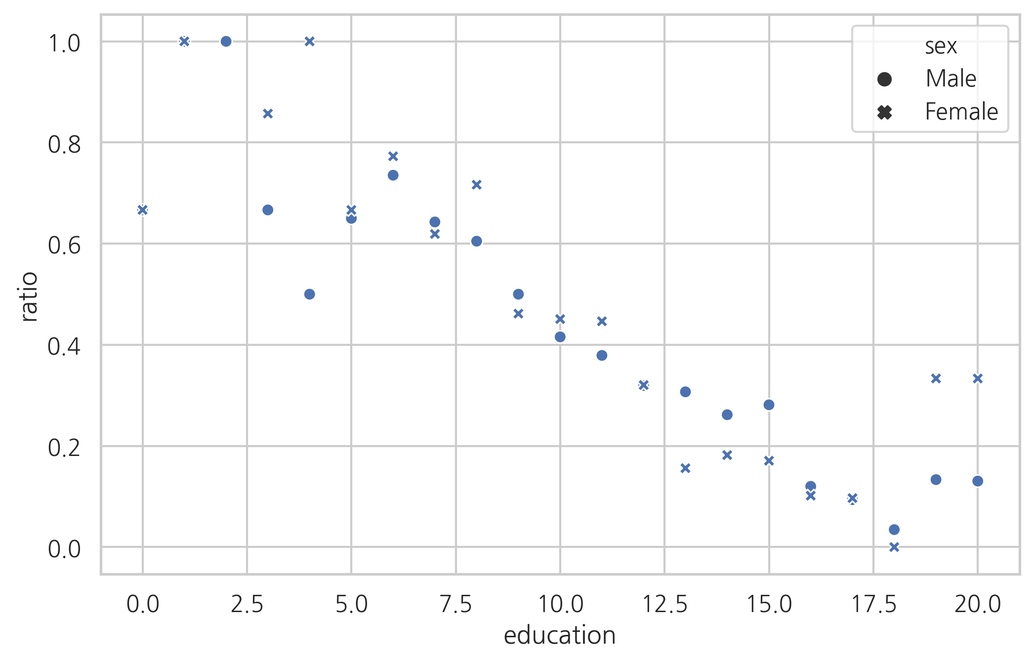
다음 데이터는 1974년도에 “여성은 가정을 보살피고 국가를 운영하는 일은 남자에게 맡겨두어야 한다.”라는 주장에 대한 찬성, 반대 입장을 조사한 결과이다. 각 열은 다음을 뜻한다.
education: 교육 기간sex: 성별agree: 찬성 인원disagree: 반대 인원ratio: 찬성 비율
data_wrole = sm.datasets.get_rdataset("womensrole", package="HSAUR")
df_wrole = data_wrole.data
df_wrole["ratio"] = df_wrole.agree / (df_wrole.agree + df_wrole.disagree)
df_wrole.tail()
| education | sex | agree | disagree | ratio | |
|---|---|---|---|---|---|
| 37 | 16 | Female | 13 | 115 | 0.101562 |
| 38 | 17 | Female | 3 | 28 | 0.096774 |
| 39 | 18 | Female | 0 | 21 | 0.000000 |
| 40 | 19 | Female | 1 | 2 | 0.333333 |
| 41 | 20 | Female | 2 | 4 | 0.333333 |
교육을 많이 받은 사람일수록 찬성 비율이 감소하는 것을 볼 수 있다.
sns.scatterplot(x="education", y="ratio", style="sex", data=df_wrole)
plt.grid(True)
plt.show()
분석 결과는 다음과 같다.
model_wrole = sm.Logit.from_formula("ratio ~ education + sex", df_wrole)
result_wrole = model_wrole.fit()
print(result_wrole.summary())
Optimization terminated successfully.
         Current function value: 0.448292
         Iterations 6
                           Logit Regression Results
==============================================================================
Dep. Variable:                  ratio   No. Observations:                   41
Model:                          Logit   Df Residuals:                       38
Method:                           MLE   Df Model:                            2
Date:                Sat, 06 Jun 2020   Pseudo R-squ.:                  0.3435
Time:                        10:01:57   Log-Likelihood:                -18.380
converged:                       True   LL-Null:                       -27.997
Covariance Type:            nonrobust   LLR p-value:                 6.660e-05
===============================================================================
                  coef    std err          z      P>|z|      [0.025      0.975]
-------------------------------------------------------------------------------
Intercept       2.0442      0.889      2.299      0.022       0.302       3.787
sex[T.Male]    -0.1968      0.736     -0.267      0.789      -1.640       1.247
education      -0.2127      0.071     -2.987      0.003      -0.352      -0.073
===============================================================================
성별은 유의하지 않다는 것을 알게되었으므로 성별을 제외하고 다시 모형을 구한다.
model_wrole2 = sm.Logit.from_formula("ratio ~ education", df_wrole)
result_wrole2 = model_wrole2.fit()
print(result_wrole2.summary())
Optimization terminated successfully.
         Current function value: 0.449186
         Iterations 6
                           Logit Regression Results
==============================================================================
Dep. Variable:                  ratio   No. Observations:                   41
Model:                          Logit   Df Residuals:                       39
Method:                           MLE   Df Model:                            1
Date:                Sat, 06 Jun 2020   Pseudo R-squ.:                  0.3422
Time:                        10:01:58   Log-Likelihood:                -18.417
converged:                       True   LL-Null:                       -27.997
Covariance Type:            nonrobust   LLR p-value:                 1.202e-05
==============================================================================
                 coef    std err          z      P>|z|      [0.025      0.975]
------------------------------------------------------------------------------
Intercept      1.9345      0.781      2.478      0.013       0.405       3.464
education     -0.2117      0.071     -2.983      0.003      -0.351      -0.073
==============================================================================
sns.scatterplot(x="education", y="ratio", data=df_wrole)
xx = np.linspace(0, 20, 100)
df_wrole_p = pd.DataFrame({"education": xx})
plt.plot(xx, result_wrole2.predict(df_wrole_p), "r-", lw=4, label="예측")
plt.legend()
plt.show()
# 연습문제 1 답
from sklearn.datasets import load_iris

iris = load_iris()
idx = np.in1d(iris.target, [0, 1])
X0 = iris.data[idx, :1]
X = sm.add_constant(X0)
y = iris.target[idx]
logit_mod = sm.Logit(y, X)
logit_res = logit_mod.fit(disp=0)
print(logit_res.summary())
                           Logit Regression Results
==============================================================================
Dep. Variable:                      y   No. Observations:                  100
Model:                          Logit   Df Residuals:                       98
Method:                           MLE   Df Model:                            1
Date:                Sat, 06 Jun 2020   Pseudo R-squ.:                  0.5368
Time:                        10:02:05   Log-Likelihood:                -32.106
converged:                       True   LL-Null:                       -69.315
Covariance Type:            nonrobust   LLR p-value:                 6.320e-18
==============================================================================
                 coef    std err          z      P>|z|      [0.025      0.975]
------------------------------------------------------------------------------
const        -27.8315      5.434     -5.122      0.000     -38.481     -17.182
x1             5.1403      1.007      5.107      0.000       3.168       7.113
==============================================================================
logit_res.params
array([-27.83145099, 5.14033614])
-logit_res.params[0] / logit_res.params[1]
5.41432510257189
y_pred = logit_res.predict(X) >= 0.5
from sklearn.metrics import confusion_matrix

confusion_matrix(y, y_pred)
array([[45,  5],
       [ 6, 44]])
from sklearn.metrics import classification_report

print(classification_report(y, y_pred))
              precision    recall  f1-score   support

           0       0.88      0.90      0.89        50
           1       0.90      0.88      0.89        50

    accuracy                           0.89       100
   macro avg       0.89      0.89      0.89       100
weighted avg       0.89      0.89      0.89       100
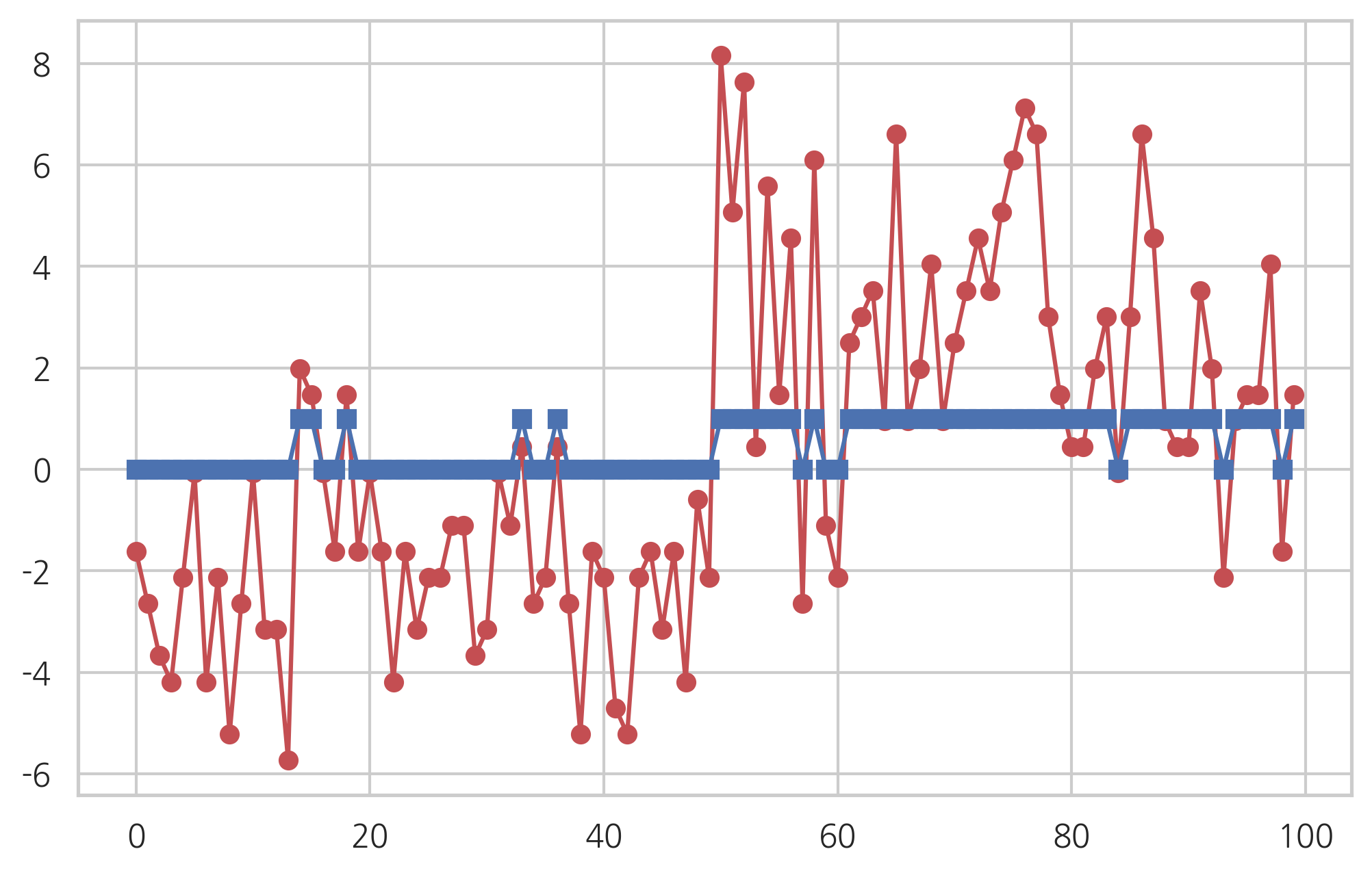
plt.plot(logit_res.fittedvalues, "ro-")
plt.plot(y_pred, "bs-")
[<matplotlib.lines.Line2D at 0x7f653c0d97f0>]
from sklearn.metrics import roc_curve

fpr, tpr, thresholds = roc_curve(y, logit_res.fittedvalues)

plt.plot(fpr, tpr, 'o-')
plt.show()
# 연습문제 2 답
from sklearn.datasets import load_iris

iris = load_iris()
idx = np.in1d(iris.target, [1, 2])
X0 = pd.DataFrame(iris.data[idx, :], columns=iris.feature_names[:])
X = sm.add_constant(X0)
y = iris.target[idx] - 1
logit_mod = sm.Logit(y, X)
logit_res = logit_mod.fit(disp=1)
print(logit_res.summary())
Optimization terminated successfully.
         Current function value: 0.059493
         Iterations 12
                           Logit Regression Results
==============================================================================
Dep. Variable:                      y   No. Observations:                  100
Model:                          Logit   Df Residuals:                       95
Method:                           MLE   Df Model:                            4
Date:                Sat, 06 Jun 2020   Pseudo R-squ.:                  0.9142
Time:                        10:02:15   Log-Likelihood:                -5.9493
converged:                       True   LL-Null:                       -69.315
Covariance Type:            nonrobust   LLR p-value:                 1.947e-26
=====================================================================================
                        coef    std err          z      P>|z|      [0.025      0.975]
-------------------------------------------------------------------------------------
const               -42.6378     25.708     -1.659      0.097     -93.024       7.748
sepal length (cm)    -2.4652      2.394     -1.030      0.303      -7.158       2.228
sepal width (cm)     -6.6809      4.480     -1.491      0.136     -15.461       2.099
petal length (cm)     9.4294      4.737      1.990      0.047       0.145      18.714
petal width (cm)     18.2861      9.743      1.877      0.061      -0.809      37.381
=====================================================================================

Possibly complete quasi-separation: A fraction 0.60 of observations can be
perfectly predicted. This might indicate that there is complete
quasi-separation. In this case some parameters will not be identified.
y_pred = logit_res.predict(X) >= 0.5
from sklearn.metrics import confusion_matrix

confusion_matrix(y, y_pred)
array([[49,  1],
       [ 1, 49]])
from sklearn.metrics import classification_report

print(classification_report(y, y_pred))
              precision    recall  f1-score   support

           0       0.98      0.98      0.98        50
           1       0.98      0.98      0.98        50

    accuracy                           0.98       100
   macro avg       0.98      0.98      0.98       100
weighted avg       0.98      0.98      0.98       100