부스팅 방법

부스트(boost) 방법은 미리 정해진 갯수의 모형 집합을 사용하는 것이 아니라 하나의 모형에서 시작하여 모형 집합에 포함할 개별 모형을 하나씩 추가한다. 모형의 집합은 위원회(commitee) \(C\)라고 하고 \(m\)개의 모형을 포함하는 위원회를 \(C_m\)으로 표시한다. 위원회에 들어가는 개별 모형을 약 분류기(weak classifier)라고 하며 \(k\)로 표시한다.

부스트 방법의 특징은 한번에 하나씩 모형을 추가한다는 것이다.

\[ C_1 = \{ k_1 \} \]

\[ C_2 = C_1 \cup k_2 = \{ k_1, k_2 \} \]

\[ C_3 = C_2 \cup k_3 = \{ k_1, k_2, k_3 \} \]

\[ \vdots \]

\[ C_m = C_{m-1} \cup k_m = \{ k_1, k_2, \ldots, k_m \} \]

그리고 \(m\)번째로 위원회에 추가할 개별 모형 \(k_m\)의 선택 기준은 그 전단계의 위원회 \(C_{m-1}\)의 성능을 보완하는 것이다.

위원회 \(C_m\)의 최종 결정은 다수결 방법을 사용하지 않고 각각의 개별 모형의 출력을 가중치 \(\alpha\)로 가중선형조합한 값을 판별 함수로 사용한다. 또한 부스트 방법은 이진 분류에만 사용할 수 있으며 \(y\)값은 1또는 -1의 값을 가진다.

\[ y = -1 \text{ or } 1 \]

\[ C_{m}(x_i) = \text{sign} \left( \alpha_1k_1(x_i) + \cdots + \alpha_{m}k_{m}(x_i) \right) \]

에이다부스트

에이다부스트(adaboost)라는 이름은 적응 부스트(adaptive boost)라는 용어에서 나왔다. 에이다부스트는 위원회에 넣을 개별 모형 \(k_m\)을 선별하는 방법으로는 학습 데이터 집합의 \(i\)번째 데이터에 가중치 \(w_i\)를 주고 분류 모형이 틀리게 예측한 데이터의 가중치를 합한 값을 손실함수 \(L\)로 사용한다. 이 손실함수를 최소화하는 모형이 \(k_m\)으로 선택된다.

\[ L_m = \sum_{i=1}^N w_{m,i} I\left(k_m(x_i) \neq y_i\right)\]

위 식에서 \(I\)는 \(k(x_i) \neq y_i\)라는 조건이 만족되면 1, 아니면 0을 가지는 지시함수(indicator function)이다. 따라서 틀린 문제에 대한 가중치의 합이다.

위원회 \(C_m\)에 포함될 개별 모형 \(k_m\)이 선택된 후에는 가중치 \(\alpha_m\)를 결정해야 한다. 이 값은 다음처럼 계산한다.

\[ \epsilon_m = \dfrac{\sum_{i=1}^N w_{m,i} I\left(k_m(x_i) \neq y_i\right)}{\sum_{i=1}^N w_{m,i}} \]

\[ \alpha_m = \frac{1}{2}\log\left( \frac{1 - \epsilon_m}{\epsilon_m}\right) \]

데이터에 대한 가중치 \(w_{m,i}\)는 최초에는(m=1)모든 데이터에 대해 같은 값을 가지지만 위원회가 증가하면서 값이 바뀐다. 가중치의 값은 지수함수를 사용하여 위원회 \(C_{m-1}\)이 맞춘 문제는 작게, 틀린 문제는 크게 확대(boosting)된다.

\[\begin{split} w_{m,i} = w_{m-1,i} \exp (-y_iC_{m-1}) = \begin{cases} w_{m-1,i}e^{-1} & \text{ if } C_{m-1} = y_i\\ w_{m-1,i}e & \text{ if } C_{m-1} \neq y_i \end{cases} \end{split}\]

\(m\)번째 멤버의 모든 후보에 대해 위 손실 함수를 적용하여 가장 값이 작은 후보를 \(m\)번째 멤버로 선정한다.

에이다부스팅은 사실 다음과 같은 손실함수를 최소화하는 \(C_m\)을 찾아가는 방법이라는 것을 증명할 수 있다.

\[ L_m = \sum_{i=1}^N \exp(−y_i C_m(x_i)) \]

개별 멤버 \(k_m\)과 위원회의 관계는

\[ C_m(x_i) = \sum_{j=1}^m \alpha_j k_j(x_i) = C_{m-1}(x_i) + \alpha_m k_m(x_i) \]

이고 이 식을 대입하면

\[\begin{split} \begin{eqnarray} L_m &=& \sum_{i=1}^N \exp(−y_i C_m(x_i)) \\ &=& \sum_{i=1}^N \exp\left(−y_iC_{m-1}(x_i) - \alpha_m y_i k_m(x_i) \right) \\ &=& \sum_{i=1}^N \exp(−y_iC_{m-1}(x_i)) \exp\left(-\alpha_m y_i k_m(x_i)\right) \\ &=& \sum_{i=1}^N w_{m,i} \exp\left(-\alpha_m y_i k_m(x_i)\right) \\ \end{eqnarray} \end{split}\]

\(y_i\)와 \(k_M(x_i)\)가 1 또는 -1값만 가질 수 있다는 점을 이용하면,

\[\begin{split} \begin{eqnarray} L_m &=& e^{-\alpha_m}\sum_{k_m(x_i) = y_i} w_{m,i} + e^{\alpha_m}\sum_{k_m(x_i) \neq y_i} w_{m,i} \\ &=& \left(e^{\alpha_m}-e^{-\alpha_m}\right) \sum_{i=1}^N w_{m,i} I\left(k_m(x_i) \neq y_i\right) + e^{-\alpha_m}\sum_{i=1}^N w_{m,i} \end{eqnarray} \end{split}\]

\(L_m\)을 최소화하려면 \(\sum_{i=1}^N w_{m,i} I\left(k_m(x_i) \neq y_i\right)\)을 최소화하는 \(k_m\) 함수를 찾은 다음 \(L_m\)을 최소화하는 \(\alpha_m\)을 찾아야 한다.

\[ \dfrac{d L_m}{d \alpha_m} = 0 \]

이 조건으로부터 \(\alpha_m\) 공식을 유도할 수 있다.

다음은 scikit-learn의 ensemble 서브패키지가 제공하는 AdaBoostClassifier 클래스를 사용하여 분류 예측을 하는 예이다. 약분류기로는 깊이가 1인 단순한 의사결정나무를 채택하였다.

여기에서는 각 표본 데이터의 가중치 값을 알아보기 위해 기존의 AdaBoostClassifier 클래스를 서브클래싱하여 가중치를 속성으로 저장하도록 수정한 모형을 사용하였다.

from sklearn.datasets import make_gaussian_quantiles
from sklearn.tree import DecisionTreeClassifier
from sklearn.ensemble import AdaBoostClassifier

X1, y1 = make_gaussian_quantiles(cov=2.,
                                 n_samples=100, n_features=2,
                                 n_classes=2, random_state=1)
X2, y2 = make_gaussian_quantiles(mean=(3, 3), cov=1.5,
                                 n_samples=200, n_features=2,
                                 n_classes=2, random_state=1)
X = np.concatenate((X1, X2))
y = np.concatenate((y1, - y2 + 1))

class MyAdaBoostClassifier(AdaBoostClassifier):
    
    def __init__(self,
                 base_estimator=None,
                 n_estimators=50,
                 learning_rate=1.,
                 algorithm='SAMME.R',
                 random_state=None):

        super(MyAdaBoostClassifier, self).__init__(
            base_estimator=base_estimator,
            n_estimators=n_estimators,
            learning_rate=learning_rate,
            random_state=random_state)
        self.sample_weight = [None] * n_estimators
        
    def _boost(self, iboost, X, y, sample_weight, random_state):
        sample_weight, estimator_weight, estimator_error = \
        super(MyAdaBoostClassifier, self)._boost(iboost, X, y, sample_weight, random_state)
        self.sample_weight[iboost] = sample_weight.copy()
        return sample_weight, estimator_weight, estimator_error
    
model_ada = MyAdaBoostClassifier(DecisionTreeClassifier(max_depth=1, random_state=0), n_estimators=20)
model_ada.fit(X, y)

def plot_result(model, title="분류결과", legend=False, s=50):
    x1_min, x1_max = X[:, 0].min() - 1, X[:, 0].max() + 1
    x2_min, x2_max = X[:, 1].min() - 1, X[:, 1].max() + 1
    xx1, xx2 = np.meshgrid(np.arange(x1_min, x1_max, 0.02), np.arange(x2_min, x2_max, 0.02))
    if isinstance(model, list):
        Y = model[0].predict(np.c_[xx1.ravel(), xx2.ravel()]).reshape(xx1.shape)
        for i in range(len(model) - 1):
            Y += model[i + 1].predict(np.c_[xx1.ravel(), xx2.ravel()]).reshape(xx1.shape)
    else:
        Y = model.predict(np.c_[xx1.ravel(), xx2.ravel()]).reshape(xx1.shape)
    cs = plt.contourf(xx1, xx2, Y, cmap=plt.cm.Paired, alpha=0.5)
    for i, n, c in zip(range(2), "01", "br"):
        idx = np.where(y == i)
        plt.scatter(X[idx, 0], X[idx, 1], c=c, s=s, alpha=0.5, label="Class %s" % n)
    plt.xlim(x1_min, x1_max)
    plt.ylim(x2_min, x2_max)
    plt.xlabel('x1')
    plt.ylabel('x2')
    plt.title(title)
    plt.colorbar(cs)
    if legend:
        plt.legend()
    plt.grid(False)

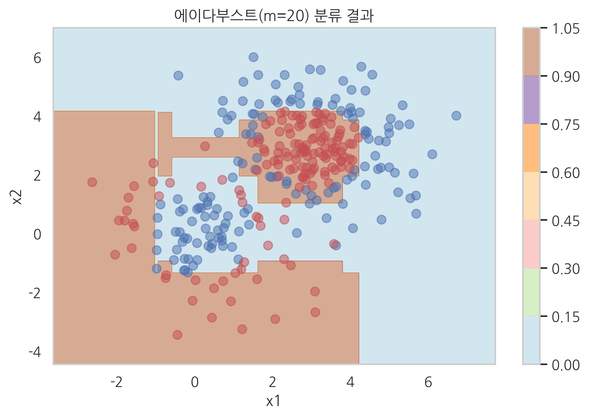
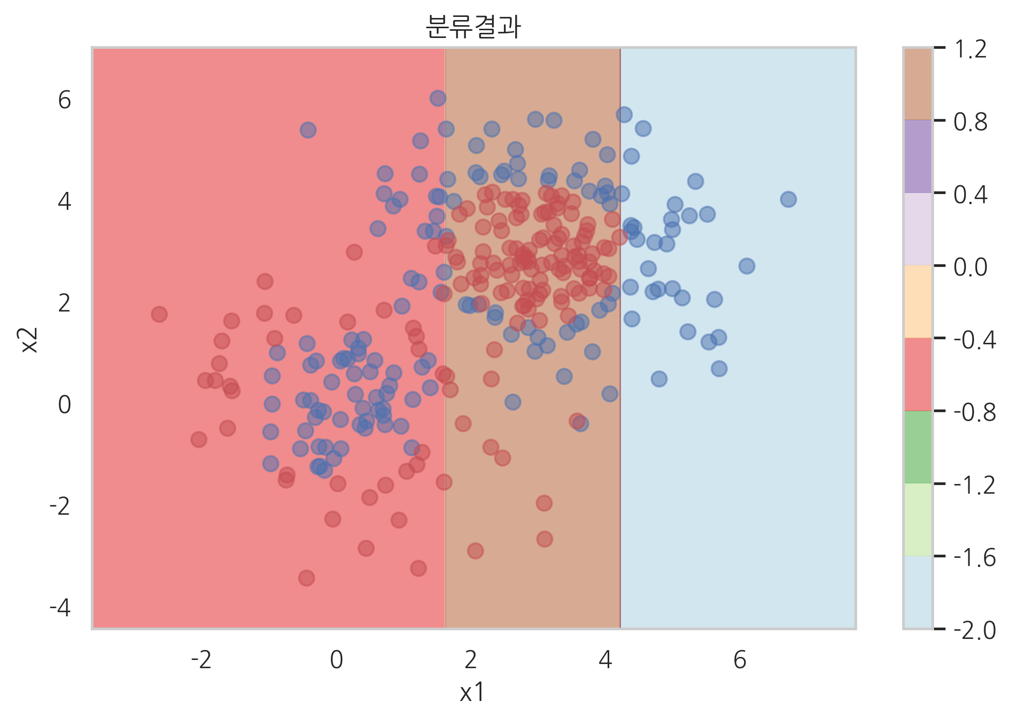
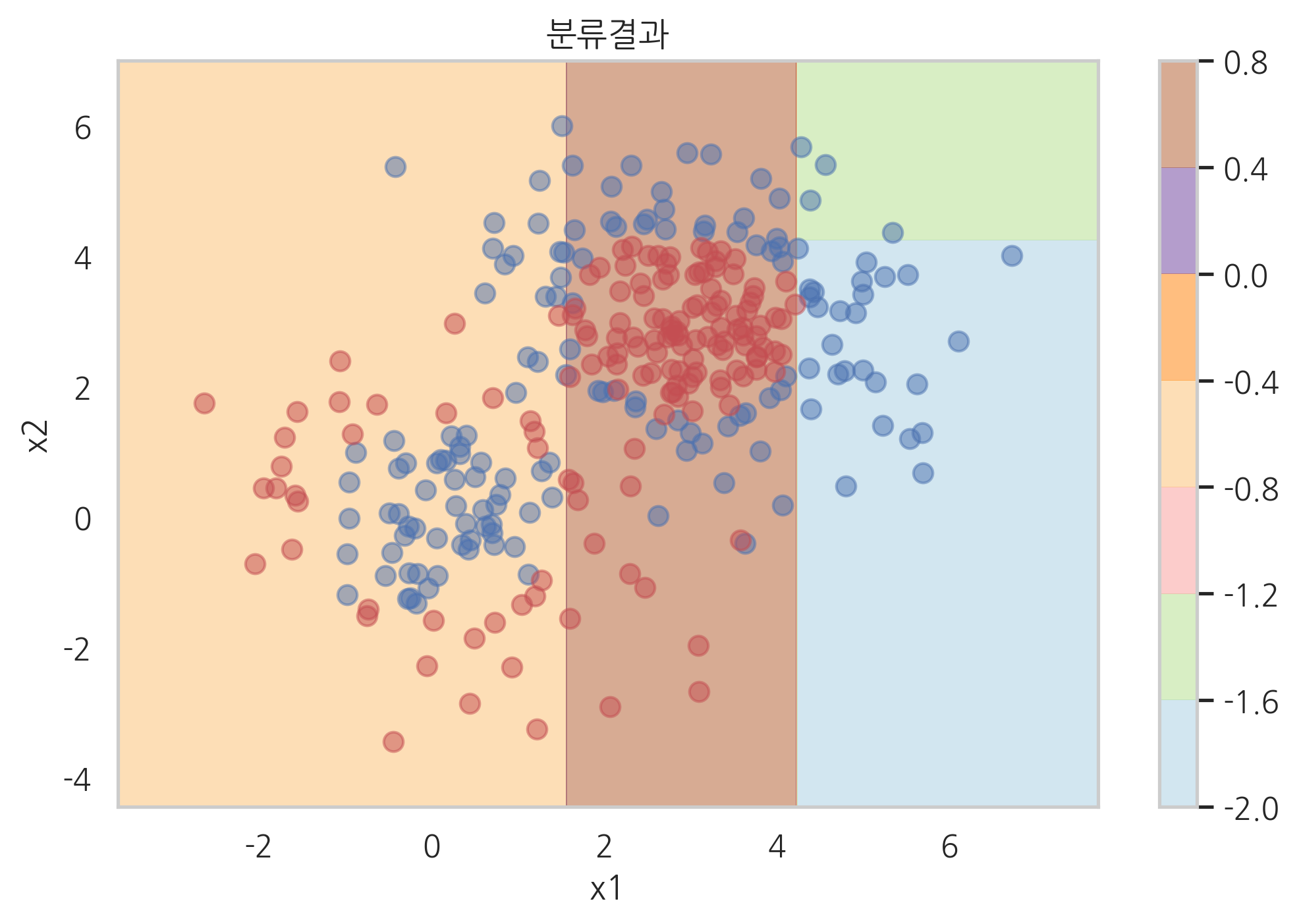
plot_result(model_ada, "에이다부스트(m=20) 분류 결과")

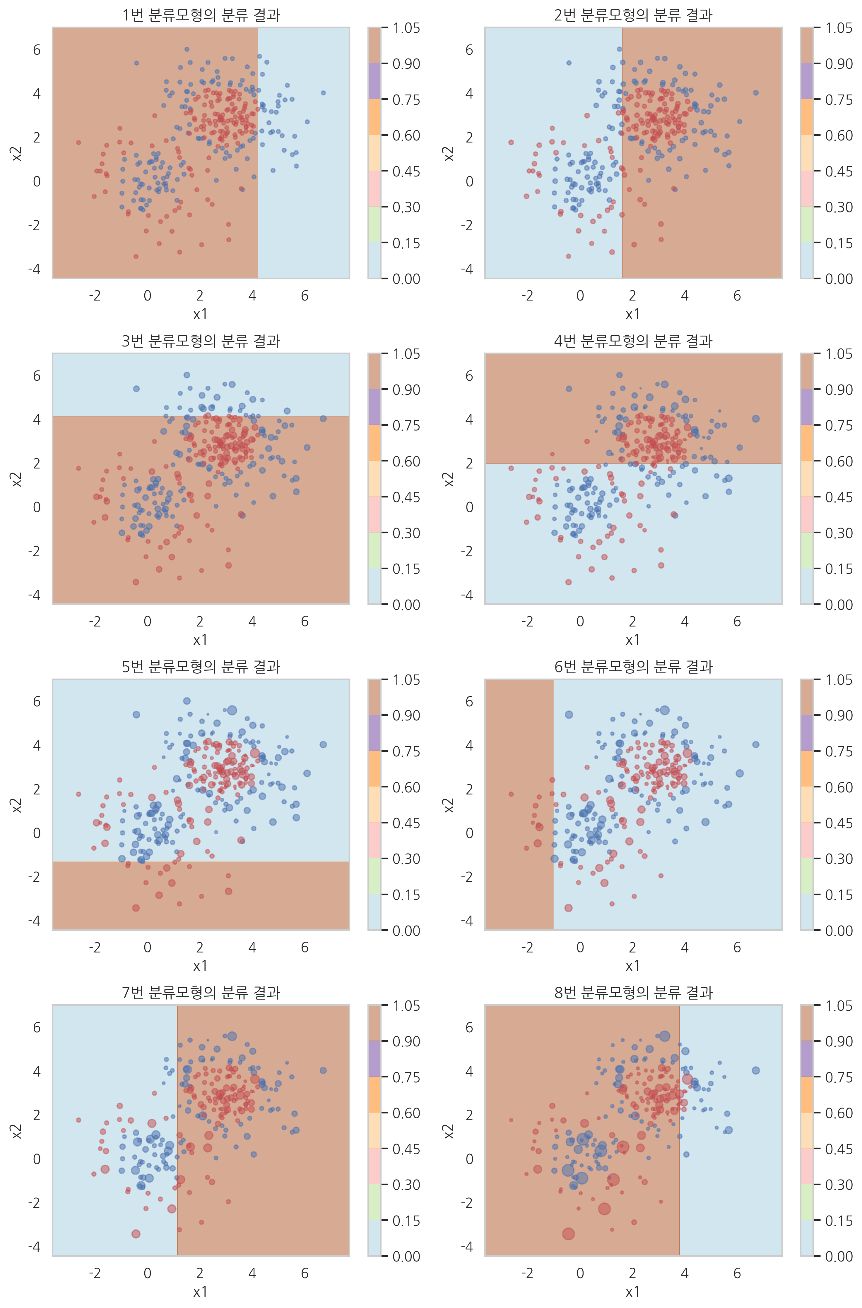
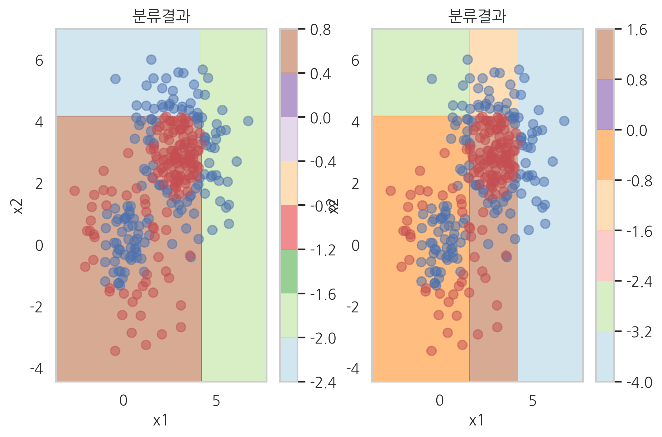
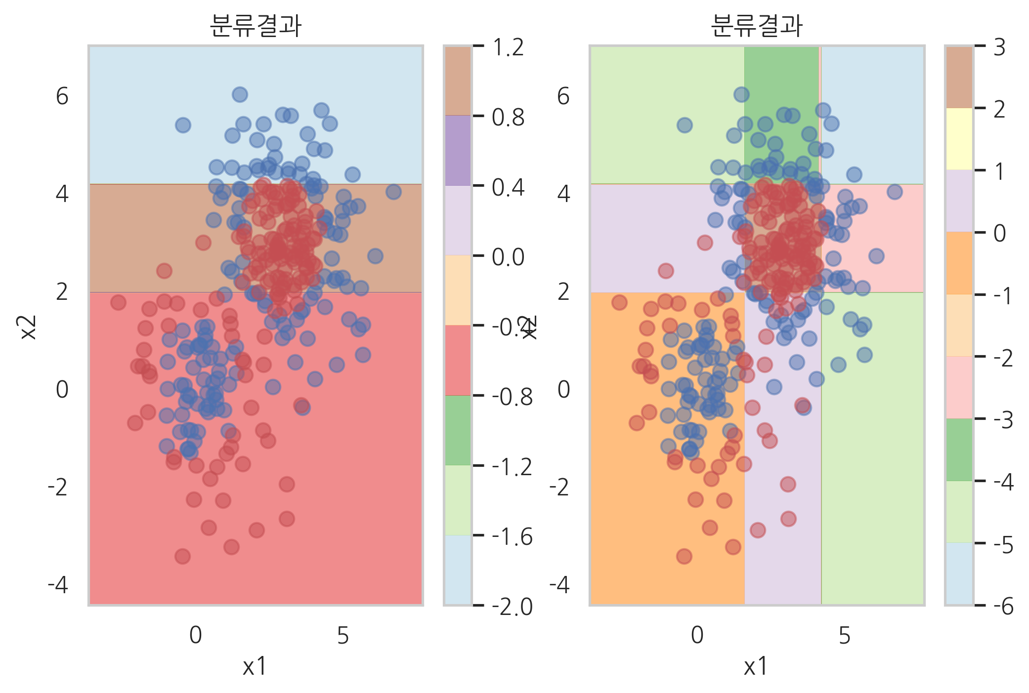
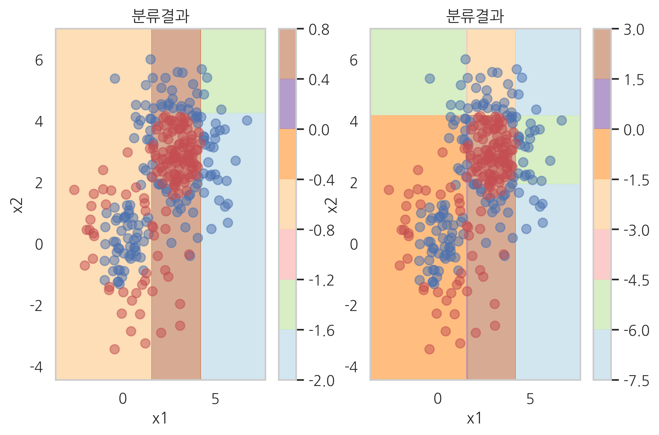
각 단계의 분류 모형에 대한 가중치 값과 분류 모형의 분류 결과를 시각화하면 다음과 같다. 데이터의 가중치는 스캐터플롯의 점의 크기로 표현하였다. 단계가 진행될 수록 가중치값의 변화가 커지는 것을 볼 수 있다.

plt.figure(figsize=(10, 15))
plt.subplot(421); 
plot_result(model_ada.estimators_[0], "1번 분류모형의 분류 결과", s=10)
plt.subplot(422); 
plot_result(model_ada.estimators_[1], "2번 분류모형의 분류 결과", s=(4000*model_ada.sample_weight[0]).astype(int))
plt.subplot(423); 
plot_result(model_ada.estimators_[2], "3번 분류모형의 분류 결과", s=(4000*model_ada.sample_weight[1]).astype(int))
plt.subplot(424); 
plot_result(model_ada.estimators_[3], "4번 분류모형의 분류 결과", s=(4000*model_ada.sample_weight[2]).astype(int))
plt.subplot(425); 
plot_result(model_ada.estimators_[4], "5번 분류모형의 분류 결과", s=(4000*model_ada.sample_weight[3]).astype(int))
plt.subplot(426); 
plot_result(model_ada.estimators_[5], "6번 분류모형의 분류 결과", s=(4000*model_ada.sample_weight[4]).astype(int))
plt.subplot(427); 
plot_result(model_ada.estimators_[6], "7번 분류모형의 분류 결과", s=(4000*model_ada.sample_weight[5]).astype(int))
plt.subplot(428); 
plot_result(model_ada.estimators_[7], "8번 분류모형의 분류 결과", s=(4000*model_ada.sample_weight[6]).astype(int))
plt.tight_layout()

에이다부스트 모형의 정규화

에이다부스트 모형이 과최적화가 되는 경우에는 학습 속도(learning rate) 조정하여 정규화를 할 수 있다. 이는 필요한 멤버의 수를 강제로 증가시켜서 과최적화를 막는 역할을 한다.

\[ C_m = C_{m-1} + \mu \alpha_m k_m \]

AdaBoostClassifier 클래스에서는 learning_rate 인수를 1보다 적게 주면 새로운 멤버의 가중치를 강제로 낮춘다.

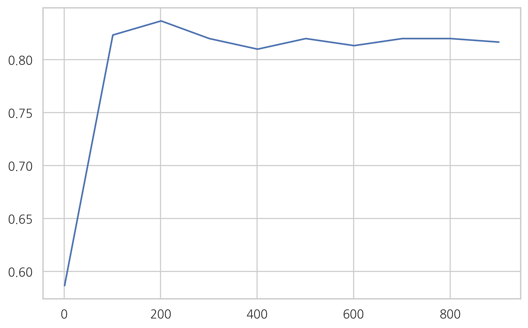
연습 문제 1

1. 위 예제에서 멤버의 수를 1000까지 100단위로 증가시키면서 성능의 변화를 살펴본다. 과최적화가 심해지는가 감소하는가?

2. 멤버의 수가 1000일 때 학습속도(learning_rate)인수를 조정하여 과최적화를 없애본다. K=5인 교차검정을 이용하여 가장 검증성능이 좋은 학습속도를 찾아라.

%%time 

from sklearn.tree import DecisionTreeClassifier
from sklearn.ensemble import AdaBoostClassifier
from sklearn.model_selection import cross_val_score

mean_test_accuracy = []
for n in np.arange(1, 1001, 100):
    model1 = AdaBoostClassifier(DecisionTreeClassifier(max_depth=1), n_estimators=n)
    mean_test_accuracy.append(cross_val_score(model1, X, y, cv=5).mean())

CPU times: user 2min 1s, sys: 1.62 s, total: 2min 2s
Wall time: 2min 4s

plt.plot(np.arange(1, 1000, 100), mean_test_accuracy)
plt.show()

그레디언트 부스트

그레이던트 부스트 모형은 변분법(calculus of variations)을 사용한 모형이다.

함수 \(f(x)\)를 최소화하는 \(x\)는 다음과 같이 gradient descent 방법으로 찾을 수 있다.

\[ x_{m} = x_{m-1} - \alpha_m \dfrac{df}{dx} \]

그레디언트 부스트 모형에서는 손실 범함수(loss functional) \(L(y, C_{m-1})\)을 최소화하는 개별 분류함수 \(k_m\)를 찾는다. 이론적으로 가장 최적의 함수는 범함수의 미분이다.

\[ C_{m} = C_{m-1} - \alpha_m \dfrac{\delta L(y, C_{m-1})}{\delta C_{m-1}} = C_{m-1} + \alpha_m k_m \]

따라서 그레디언트 부스트 모형은 분류/회귀 문제에 상관없이 개별 멤버 모형으로 회귀분석 모형을 사용한다. 가장 많이 사용되는 회귀분석 모형은 의사결정 회귀나무(decision tree regression model) 모형이다.

그레디언트 부스트 모형에서는 다음과 같은 과정을 반복하여 멤버와 그 가중치를 계산한다.

1. \(-\tfrac{\delta L(y, C_m)}{\delta C_m}\) 를 목표값으로 개별 멤버 모형 \(k_m\) 을 찾는다.

2. \( \left( y - (C_{m-1} + \alpha_m k_m) \right)^2 \) 를 최소화하는 스텝사이즈 \(\alpha_m\) 을 찾는다.

3. \(C_m = C_{m-1} + \alpha_m k_m\) 최종 모형을 갱신한다.

만약 손실 범함수가 오차 제곱 형태라면

\[ L(y, C_{m-1}) = \dfrac{1}{2}(y - C_{m-1})^2 \]

범함수의 미분은 실제 목푯값 \(y\)와 \(C_{m-1}\)과의 차이 즉, 잔차(residual)가 된다.

\[ -\dfrac{dL(y, C_m)}{dC_m} = y - C_{m-1} \]

from sklearn.ensemble import GradientBoostingClassifier

model_grad = GradientBoostingClassifier(n_estimators=100, max_depth=2, random_state=0)

%%time
model_grad.fit(X, y)

CPU times: user 50 ms, sys: 0 ns, total: 50 ms
Wall time: 50.4 ms

GradientBoostingClassifier(criterion='friedman_mse', init=None,
                           learning_rate=0.1, loss='deviance', max_depth=2,
                           max_features=None, max_leaf_nodes=None,
                           min_impurity_decrease=0.0, min_impurity_split=None,
                           min_samples_leaf=1, min_samples_split=2,
                           min_weight_fraction_leaf=0.0, n_estimators=100,
                           n_iter_no_change=None, presort='auto',
                           random_state=0, subsample=1.0, tol=0.0001,
                           validation_fraction=0.1, verbose=0,
                           warm_start=False)

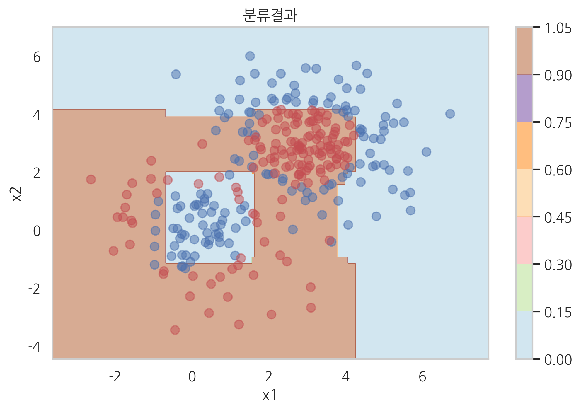
plot_result(model_grad)

plot_result(model_grad.estimators_[0][0])

plt.subplot(121)
plot_result(model_grad.estimators_[1][0])
plt.subplot(122)
plot_result([model_grad.estimators_[0][0], model_grad.estimators_[1][0]])

plt.subplot(121)
plot_result(model_grad.estimators_[2][0])
plt.subplot(122)
plot_result([model_grad.estimators_[0][0], 
             model_grad.estimators_[1][0],
             model_grad.estimators_[2][0]])

plt.subplot(121)
plot_result(model_grad.estimators_[3][0])
plt.subplot(122)
plot_result([model_grad.estimators_[0][0], 
             model_grad.estimators_[1][0],
             model_grad.estimators_[2][0],
             model_grad.estimators_[3][0]])

plot_result(model_grad.estimators_[3][0])

XGBoost 라이브러리

import xgboost

model_xgb = xgboost.XGBClassifier(n_estimators=100, max_depth=1, random_state=0)

%%time
model_xgb.fit(X, y)

CPU times: user 20 ms, sys: 0 ns, total: 20 ms
Wall time: 12.2 ms

XGBClassifier(base_score=0.5, booster='gbtree', colsample_bylevel=1,
              colsample_bynode=1, colsample_bytree=1, gamma=0,
              learning_rate=0.1, max_delta_step=0, max_depth=1,
              min_child_weight=1, missing=None, n_estimators=100, n_jobs=1,
              nthread=None, objective='binary:logistic', random_state=0,
              reg_alpha=0, reg_lambda=1, scale_pos_weight=1, seed=None,
              silent=None, subsample=1, verbosity=1)

plot_result(model_xgb)

LightGBM 라이브러리

import lightgbm

model_lgbm = lightgbm.LGBMClassifier(n_estimators=100, max_depth=1, random_state=0)

%%time
model_lgbm.fit(X, y)

CPU times: user 10 ms, sys: 0 ns, total: 10 ms
Wall time: 15 ms

LGBMClassifier(boosting_type='gbdt', class_weight=None, colsample_bytree=1.0,
               importance_type='split', learning_rate=0.1, max_depth=1,
               min_child_samples=20, min_child_weight=0.001, min_split_gain=0.0,
               n_estimators=100, n_jobs=-1, num_leaves=31, objective=None,
               random_state=0, reg_alpha=0.0, reg_lambda=0.0, silent=True,
               subsample=1.0, subsample_for_bin=200000, subsample_freq=0)

plot_result(model_lgbm)

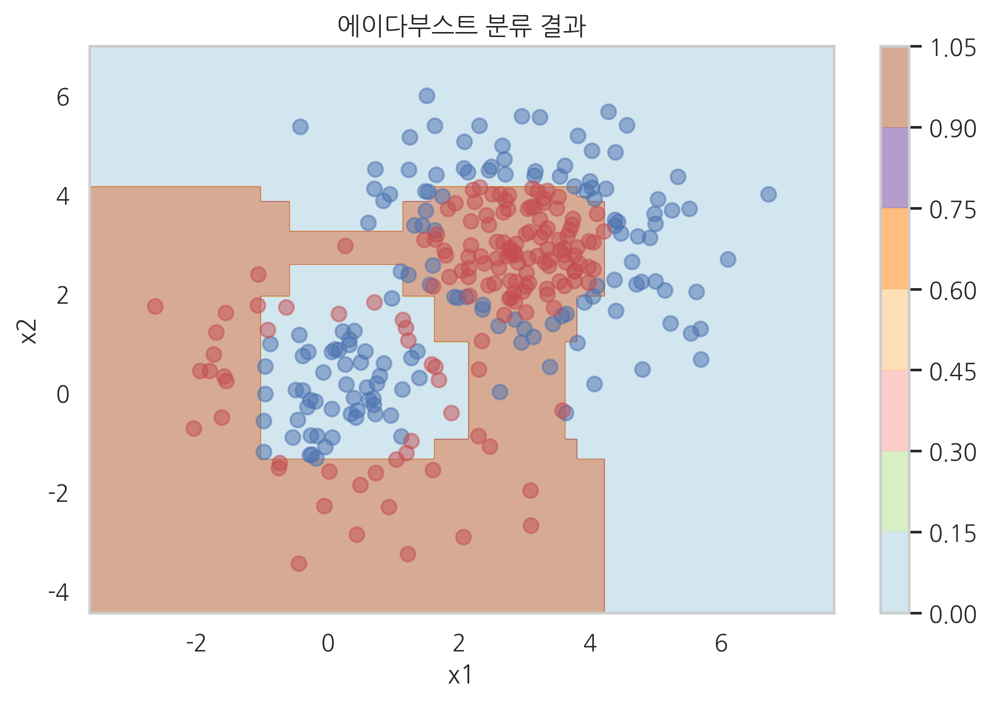
## 연습문제 1
model = AdaBoostClassifier(
    DecisionTreeClassifier(max_depth=1, random_state=0), 
    n_estimators=200, learning_rate=0.1).fit(X, y)
plot_result(model, "에이다부스트 분류 결과")