4.4 범주형 독립변수#
이 절에서는 범주형 독립변수를 가지는 경우의 회귀분석모형을 공부한다.
범주형 변수가 하나인 경우#
\(x_1, x_2, \ldots, x_D\)라는 \(D\)개의 독립변수를 가지는 선형회귀모형을 생각하자.
여기에서 \(x_1\)이라는 독립변수만 범주형 변수이고 ‘A’과 ‘B’라는 두 가지의 범주값을 가질 수 있다고 하자.
가장 간단한 방법은 전체 데이터를 \(x_1=A\)인 데이터와 \(x_2=B\)인 데이터 두 그룹으로 나누어 각각의 데이터에 대한 선형회귀모형을 만드는 것이다. 즉 다음과 같은 2개의 선형회귀모형을 만든다.
그런데 올바른 선형회귀모형에서는 \(x_1\)이 아닌 다른 변수 예를 들어 \(x_2\)의 값이 변할 때 \(y\)값이 변화하는 정도, 즉 가중치 \(w_2\)는 \(x_1\)의 값이 A이든 B든 같아야 한다. 하지만 위와 같은 두 개의 선형회귀모형을 만들면 \(w_2\)의 값이 \(w_{A,2}\)와 \(w_{B,2}\)라는 두 가지의 다른 값이 나오므로 위 모형은 적당하지 않다.
더미변수 방법은 범주형 변수 \(x_1\)을 \(d_{1A}, d_{1B}\)라는 두 개의 더미변수로 바꾸는 것이다. 더미변수는 상수항을 포함하기 때문에 더미변수로 변환하면 상수항은 없어진다.
더미변수가 2개인 이유는 더미변수가 가질 수 있는 범주값이 2개이기 때문이다. 범주값이 \(K\)개이면 범주형 변수 \(x_1\)을 \(d_{11}, \ldots, d_{1K}\)라는 \(K\)개의 더미변수로 바꾸어야 한다.
풀랭크 방식#
풀랭크(full-rank) 방식에서는 더미변수의 값을 원핫인코딩(one-hot-encoding) 방식으로 지정한다. 즉 범주값이 2가지인 경우에는
이 된다. 이 값을 대입하면 더미변수의 가중치는 상수항이 된다.
위 수식은 \(x_1=A\)인 데이터에 대해서는 \(\hat{y} = w_{1A} + w_2 x_2 + \cdots + w_D x_D\) 모형을 사용하고 \(x_1=B\)인 데이터에 대해서는 \(\hat{y} = w_{1B} + w_2 x_2 + \cdots + w_D x_D\) 모형을 사용하게 된다는 뜻이다. 이렇게 하면 범주값이 달라졌을 때 상수항만 달라지고 다른 독립변수의 가중치(영향)는 같은 모형이 된다.
%load_ext tikzmagic
%%tikz -p kotex,pgfplots -l arrows.meta,calc -s 2000,1200 -f png

\coordinate (leftbottom) at (1,0);
\coordinate (righttop) at (12,6);
\fill[white,use as bounding box] (leftbottom) rectangle (righttop);
\draw[help lines, white] (leftbottom) grid (righttop);
\tikzset{
    >=stealth,font={\ttfamily\large}
}

\node (origin) at (3,1) {};
\draw[->] (3,0.3)--(3,5);
\node at (3,5.3) {$y$};
\draw[->] (2.5,1)--(10,1);
\node at (10.4,1) {$x_2$};
\draw[line width=1pt] (2.5,1.91)--(9,3);
\node at (9.8,3.1) {$x_1=A$};
\node(w1A) at (3,2) {};
\draw[fill] (w1A) circle (2pt);
\node at (2.6,2.3) {$w_{1A}$};
\draw[line width=1pt] (2.5,3.91)--(9,5);
\node at (9.8,5.1) {$x_1=B$};
\node(w1B) at (3,4) {};
\draw[fill] (w1B) circle (2pt);
\node at (2.6,4.3) {$w_{1B}$};
\draw[dotted, line width=1pt] (origin.center) edge[bend right] (w1A.center);
\draw[dotted, line width=1pt] (origin.center) edge[bend right] (w1B.center);
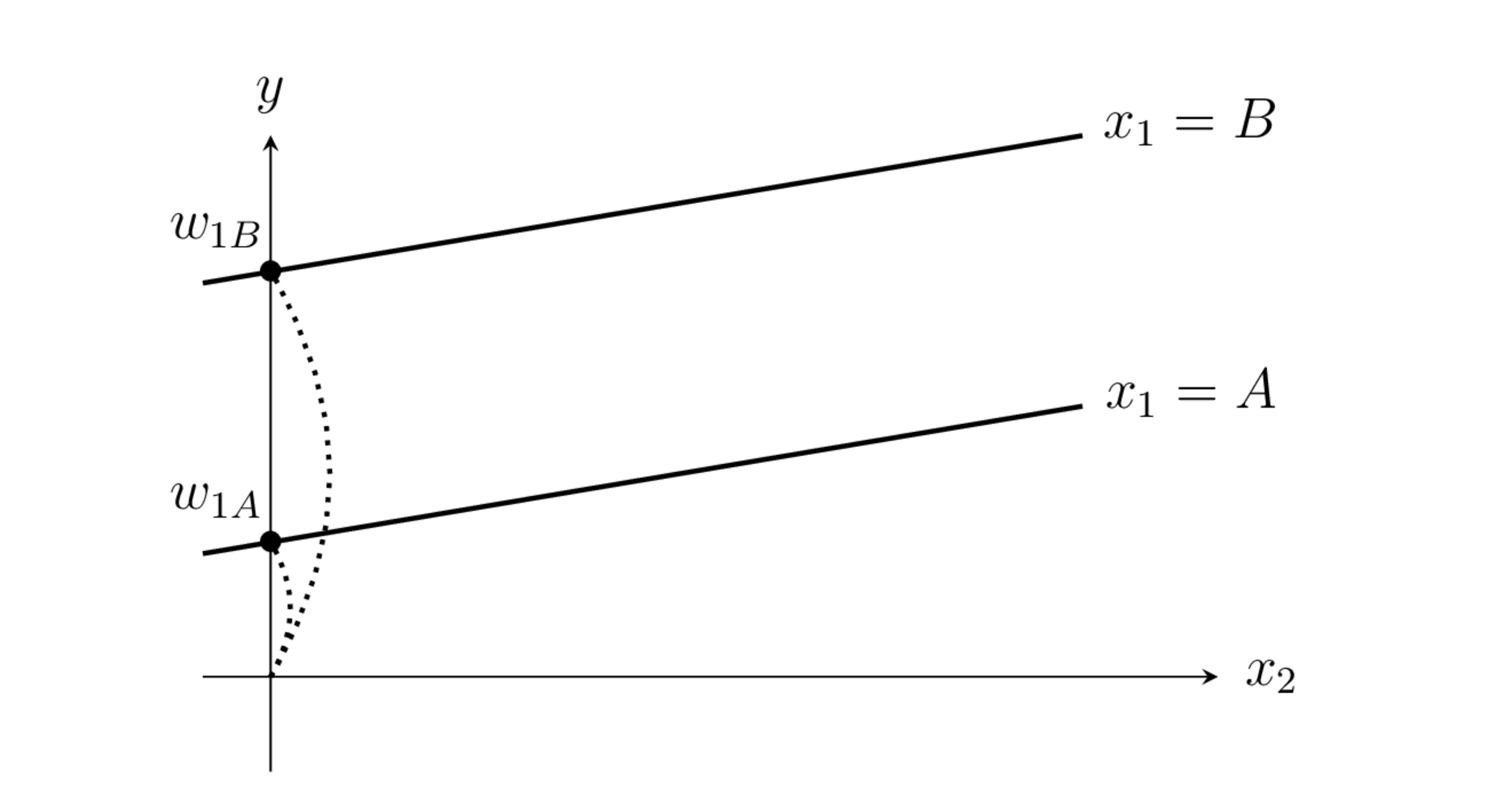
그림 : 풀랭크 방식 더미변수 가중치의 의미
선형회귀모형에 범주형 독립변수가 있으면 더미변수의 가중치 이외에 별도의 상수항이 있으면 안된다. 만약 위의 모형에서 별도의 상수항 \(w_0\)이 존재한다면 모형은 다음처럼 될 것이다.
이 경우에는 \(w_0 + w_{1A}\)나 \(w_0 + w_{1B}\)의 값은 구할 수 있어도 \(w_0\) 값과 \(w_{1A}\) 값을 분리할 수는 없다. 범주형 독립변수가 있으면 상수항은 포함시키지 않는다.
축소랭크 방식#
축소랭크(reduced-rank) 방식에서는 특정한 하나의 범주값을 기준값(reference, baseline)으로 하고 기준값에 대응하는 더미변수의 가중치는 항상 1으로 놓는다. 다른 범주형 값을 가지는 경우는 기준값에 추가적인 특성이 있는 것으로 간주한다. 예를 들어 다음 축소랭크 방식은 \(x_1=A\)를 기준값으로 하는 경우이다.
반대로 \(x_1=B\)를 기준값으로 하면 다음과 같아진다.
이 값을 대입하면 기준값인 더미변수의 가중치는 상수항이 되고 나머지 더미변수의 가중치는 그 상수항에 추가적으로 더해지는 상수항이 된다. \(x_1=A\)를 기준값으로 하는 경우에는 다음과 같다.
%%tikz -p kotex,pgfplots -l arrows.meta,calc -s 2000,1200 -f png

\coordinate (leftbottom) at (1,0);
\coordinate (righttop) at (12,6);
\fill[white,use as bounding box] (leftbottom) rectangle (righttop);
\draw[help lines, white] (leftbottom) grid (righttop);
\tikzset{
    >=stealth,font={\ttfamily\large}
}

\node (origin) at (3,1) {};
\draw[->] (3,0.3)--(3,5);
\node at (3,5.3) {$y$};
\draw[->] (2.5,1)--(10,1);
\node at (10.4,1) {$x_2$};
\draw[line width=1pt] (2.5,1.91)--(9,3);
\node at (9.8,3.1) {$x_1=A$};
\node(w1A) at (3,2) {};
\draw[fill] (w1A) circle (2pt);
\node at (2.6,2.3) {$w_{1A}$};
\draw[line width=1pt] (2.5,3.91)--(9,5);
\node at (9.8,5.1) {$x_1=B$};
\node(w1B) at (3,4) {};
\draw[fill] (w1B) circle (2pt);
\node at (2.8,4.4) {$w_{1A} + w_{1B}$};
\draw[dotted, line width=1pt] (origin.center) edge[bend right] (w1A.center);
\draw[dotted, line width=1pt] (w1A.center) edge[bend right] (w1B.center);
\node at (3.8,3) {$w_{1B}$};
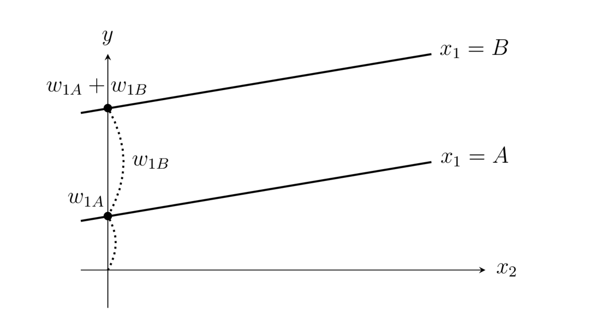
그림 : 축소랭크 방식 더미변수 가중치의 의미
예제#
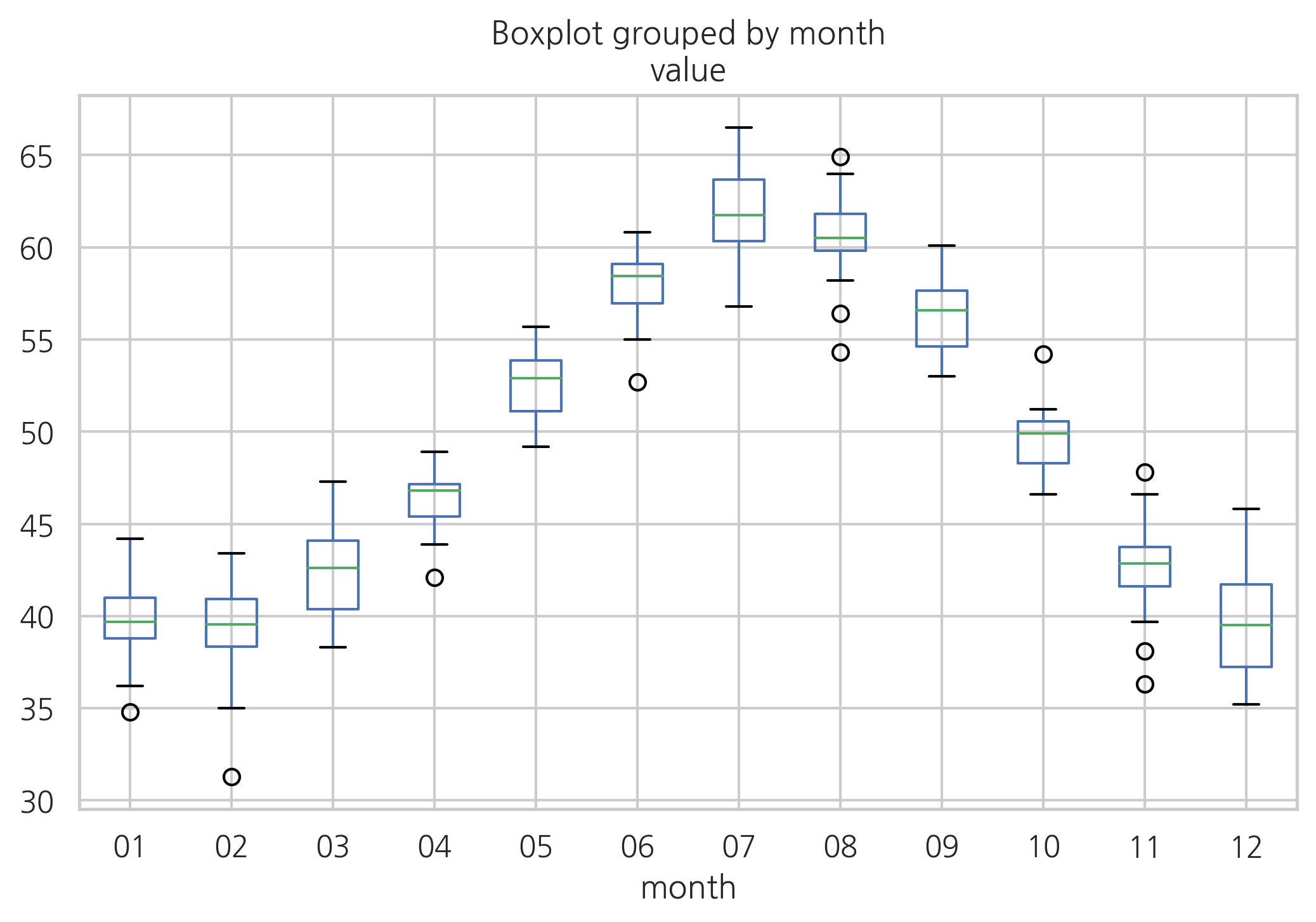
다음 데이터는 1920년부터 1939년 사이의 노팅엄(Nottingham)지역 월 평균 기온이다. 이 데이터에서 독립변수는 월(monath)이며 범주값으로 처리한다. value로 표기된 값이 종속변수인 해당 월의 평균 기온이다. 분석의 목적은 독립변수인 월 값을 이용하여 종속변수인 월 평균 기온을 예측하는 것이다. 우선 다음 코드를 사용하여 데이터 전처리를 한다.
import datetime
from calendar import isleap

def convert_partial_year(number):
    "연 단위 숫자에서 날짜를 계산하는 코드"
    year = int(number)
    d = datetime.timedelta(days=(number - year) * (365 + isleap(year)))
    day_one = datetime.datetime(year, 1, 1)
    date = d + day_one
    return date

df_nottem = sm.datasets.get_rdataset("nottem").data
df_nottem["date0"] = df_nottem[["time"]].applymap(convert_partial_year)
df_nottem["date"] = pd.DatetimeIndex(df_nottem["date0"]).round('60min') + datetime.timedelta(seconds=3600*24)
df_nottem["month"] = df_nottem["date"].dt.strftime("%m").astype('category')
del df_nottem["date0"], df_nottem["date"]
df_nottem.tail()
| time | value | month | |
|---|---|---|---|
| 235 | 1939.583333 | 61.8 | 08 |
| 236 | 1939.666667 | 58.2 | 09 |
| 237 | 1939.750000 | 46.7 | 10 |
| 238 | 1939.833333 | 46.6 | 11 |
| 239 | 1939.916667 | 37.8 | 12 |
월과 기온의 관계를 박스플롯으로 시각화하면 다음과 같다.
df_nottem.boxplot("value", "month")
plt.show()
회귀분석 모형은 다음과 같다. \(x\)는 월을 나타내는 독립변수, \(\hat{y}\)은 월 평균기온을 나타내는 종속변수다.
\(x\)를 풀랭크 방식으로 더미변수화하면 다음과 같은 모형이 된다. 이 식에서 \(d_i\)는 \(i\)월을 지시하는 더미변수다.
더미변수의 값을 대입하면 다음과 같다.
따라서 \(w_i\)는 \(i\)월의 기온의 표본평균값으로 계산된다.
statsmodels 패키지의 OLS 클래스를 사용하면 다음과 같이 회귀분석을 할 수 있다. 월 데이터가 숫자이므로 연속값으로 인식하지 않도록 C() 연산자를 사용하였다.
model = sm.OLS.from_formula("value ~ C(month) + 0", df_nottem)
result = model.fit()
print(result.summary())
                            OLS Regression Results
==============================================================================
Dep. Variable:                  value   R-squared:                       0.930
Model:                            OLS   Adj. R-squared:                  0.927
Method:                 Least Squares   F-statistic:                     277.3
Date:                Wed, 30 Oct 2019   Prob (F-statistic):          2.96e-125
Time:                        19:54:19   Log-Likelihood:                -535.82
No. Observations:                 240   AIC:                             1096.
Df Residuals:                     228   BIC:                             1137.
Df Model:                          11
Covariance Type:            nonrobust
================================================================================
                   coef    std err          t      P>|t|      [0.025      0.975]
--------------------------------------------------------------------------------
C(month)[01]    39.6950      0.518     76.691      0.000      38.675      40.715
C(month)[02]    39.1900      0.518     75.716      0.000      38.170      40.210
C(month)[03]    42.1950      0.518     81.521      0.000      41.175      43.215
C(month)[04]    46.2900      0.518     89.433      0.000      45.270      47.310
C(month)[05]    52.5600      0.518    101.547      0.000      51.540      53.580
C(month)[06]    58.0400      0.518    112.134      0.000      57.020      59.060
C(month)[07]    61.9000      0.518    119.592      0.000      60.880      62.920
C(month)[08]    60.5200      0.518    116.926      0.000      59.500      61.540
C(month)[09]    56.4800      0.518    109.120      0.000      55.460      57.500
C(month)[10]    49.4950      0.518     95.625      0.000      48.475      50.515
C(month)[11]    42.5800      0.518     82.265      0.000      41.560      43.600
C(month)[12]    39.5300      0.518     76.373      0.000      38.510      40.550
==============================================================================
Omnibus:                        5.430   Durbin-Watson:                   1.529
Prob(Omnibus):                  0.066   Jarque-Bera (JB):                5.299
Skew:                          -0.281   Prob(JB):                       0.0707
Kurtosis:                       3.463   Cond. No.                         1.00
==============================================================================

Warnings:
[1] Standard Errors assume that the covariance matrix of the errors is correctly specified.
1월을 기준월로 하는 축소랭크 방식을 사용하면 더미변수는 다음과 같다.
포뮬러 문자열에서 +0을 제외하면 축소랭크 방식을 사용한다. 이 때는 1월의 평균 기온을 기준으로 각 월의 평균 기온이 1월보다 얼마나 더 높은지를 나타내는 값이 회귀모형의 계수가 된다.
model = sm.OLS.from_formula("value ~ C(month)", df_nottem)
result = model.fit()
print(result.summary())
                            OLS Regression Results
==============================================================================
Dep. Variable:                  value   R-squared:                       0.930
Model:                            OLS   Adj. R-squared:                  0.927
Method:                 Least Squares   F-statistic:                     277.3
Date:                Wed, 30 Oct 2019   Prob (F-statistic):          2.96e-125
Time:                        19:54:19   Log-Likelihood:                -535.82
No. Observations:                 240   AIC:                             1096.
Df Residuals:                     228   BIC:                             1137.
Df Model:                          11
Covariance Type:            nonrobust
==================================================================================
                     coef    std err          t      P>|t|      [0.025      0.975]
----------------------------------------------------------------------------------
Intercept         39.6950      0.518     76.691      0.000      38.675      40.715
C(month)[T.02]    -0.5050      0.732     -0.690      0.491      -1.947       0.937
C(month)[T.03]     2.5000      0.732      3.415      0.001       1.058       3.942
C(month)[T.04]     6.5950      0.732      9.010      0.000       5.153       8.037
C(month)[T.05]    12.8650      0.732     17.575      0.000      11.423      14.307
C(month)[T.06]    18.3450      0.732     25.062      0.000      16.903      19.787
C(month)[T.07]    22.2050      0.732     30.335      0.000      20.763      23.647
C(month)[T.08]    20.8250      0.732     28.450      0.000      19.383      22.267
C(month)[T.09]    16.7850      0.732     22.931      0.000      15.343      18.227
C(month)[T.10]     9.8000      0.732     13.388      0.000       8.358      11.242
C(month)[T.11]     2.8850      0.732      3.941      0.000       1.443       4.327
C(month)[T.12]    -0.1650      0.732     -0.225      0.822      -1.607       1.277
==============================================================================
Omnibus:                        5.430   Durbin-Watson:                   1.529
Prob(Omnibus):                  0.066   Jarque-Bera (JB):                5.299
Skew:                          -0.281   Prob(JB):                       0.0707
Kurtosis:                       3.463   Cond. No.                         12.9
==============================================================================

Warnings:
[1] Standard Errors assume that the covariance matrix of the errors is correctly specified.
보스턴 집값 데이터의 범주형 변수#
보스턴 집값 데이터는 CHAS라는 범주형 변수가 있고 이 변수는 0과 1 두 개의 값을 가진다.
만약 보스턴 집값 데이터에서 상수값 가중치를 가지는 모형을 만들면 축소 랭크 방식으로 더미변수 변환되어 있는 것과 같다. 즉 다음과 같은 두 개의 모형을 각각 회귀분석하는 경우라고 볼 수 있다.
CHAS= 1 인 경우, $\( y = (w_0 + w_{\text{CHAS}}) + w_{\text{CRIM}} \text{CRIM} + w_{\text{ZN}} \text{ZN} + \cdots \)$CHAS= 0 인 경우, $\( y = w_0 + w_{\text{CRIM}} \text{CRIM} + w_{\text{ZN}} \text{ZN} + \cdots \)$
from sklearn.datasets import load_boston

boston = load_boston()

dfX = pd.DataFrame(boston.data, columns=boston.feature_names)
dfy = pd.DataFrame(boston.target, columns=["MEDV"])
df_boston = pd.concat([dfX, dfy], axis=1)

model1 = sm.OLS.from_formula("MEDV ~ " + "+".join(boston.feature_names), data=df_boston)
result1 = model1.fit()
print(result1.summary())
                            OLS Regression Results
==============================================================================
Dep. Variable:                   MEDV   R-squared:                       0.741
Model:                            OLS   Adj. R-squared:                  0.734
Method:                 Least Squares   F-statistic:                     108.1
Date:                Wed, 30 Oct 2019   Prob (F-statistic):          6.72e-135
Time:                        19:54:19   Log-Likelihood:                -1498.8
No. Observations:                 506   AIC:                             3026.
Df Residuals:                     492   BIC:                             3085.
Df Model:                          13
Covariance Type:            nonrobust
==============================================================================
                 coef    std err          t      P>|t|      [0.025      0.975]
------------------------------------------------------------------------------
Intercept     36.4595      5.103      7.144      0.000      26.432      46.487
CRIM          -0.1080      0.033     -3.287      0.001      -0.173      -0.043
ZN             0.0464      0.014      3.382      0.001       0.019       0.073
INDUS          0.0206      0.061      0.334      0.738      -0.100       0.141
CHAS           2.6867      0.862      3.118      0.002       0.994       4.380
NOX          -17.7666      3.820     -4.651      0.000     -25.272     -10.262
RM             3.8099      0.418      9.116      0.000       2.989       4.631
AGE            0.0007      0.013      0.052      0.958      -0.025       0.027
DIS           -1.4756      0.199     -7.398      0.000      -1.867      -1.084
RAD            0.3060      0.066      4.613      0.000       0.176       0.436
TAX           -0.0123      0.004     -3.280      0.001      -0.020      -0.005
PTRATIO       -0.9527      0.131     -7.283      0.000      -1.210      -0.696
B              0.0093      0.003      3.467      0.001       0.004       0.015
LSTAT         -0.5248      0.051    -10.347      0.000      -0.624      -0.425
==============================================================================
Omnibus:                      178.041   Durbin-Watson:                   1.078
Prob(Omnibus):                  0.000   Jarque-Bera (JB):              783.126
Skew:                           1.521   Prob(JB):                    8.84e-171
Kurtosis:                       8.281   Cond. No.                     1.51e+04
==============================================================================

Warnings:
[1] Standard Errors assume that the covariance matrix of the errors is correctly specified.
[2] The condition number is large, 1.51e+04. This might indicate that there are
strong multicollinearity or other numerical problems.
반대로 보스턴 집값 데이터에서 상수값 가중치를 가지지 않는 모형을 만들면 풀 랭크 방식으로 더미변수 변환되어 있는 것과 같다. 즉 다음과 같은 두 개의 모형을 각각 회귀분석하는 경우라고 볼 수 있다.
CHAS= 1 인 경우, $\( y = w_{\text{CHAS=0}}) + w_{\text{CRIM}} \text{CRIM} + w_{\text{ZN}} \text{ZN} + \cdots \)$CHAS= 0 인 경우, $\( y = w_{\text{CHAS=1}}) \text{CRIM} + w_{\text{ZN}} \text{ZN} + \cdots \)$
feature_names = list(boston.feature_names)
feature_names.remove("CHAS")
feature_names = [name for name in feature_names] + ["C(CHAS)"]
model2 = sm.OLS.from_formula("MEDV ~ 0 + " + "+".join(feature_names), data=df_boston)
result2 = model2.fit()
print(result2.summary())
                            OLS Regression Results
==============================================================================
Dep. Variable:                   MEDV   R-squared:                       0.741
Model:                            OLS   Adj. R-squared:                  0.734
Method:                 Least Squares   F-statistic:                     108.1
Date:                Wed, 30 Oct 2019   Prob (F-statistic):          6.72e-135
Time:                        19:54:19   Log-Likelihood:                -1498.8
No. Observations:                 506   AIC:                             3026.
Df Residuals:                     492   BIC:                             3085.
Df Model:                          13
Covariance Type:            nonrobust
================================================================================
                   coef    std err          t      P>|t|      [0.025      0.975]
--------------------------------------------------------------------------------
C(CHAS)[0.0]    36.4595      5.103      7.144      0.000      26.432      46.487
C(CHAS)[1.0]    39.1462      5.153      7.597      0.000      29.023      49.270
CRIM            -0.1080      0.033     -3.287      0.001      -0.173      -0.043
ZN               0.0464      0.014      3.382      0.001       0.019       0.073
INDUS            0.0206      0.061      0.334      0.738      -0.100       0.141
NOX            -17.7666      3.820     -4.651      0.000     -25.272     -10.262
RM               3.8099      0.418      9.116      0.000       2.989       4.631
AGE              0.0007      0.013      0.052      0.958      -0.025       0.027
DIS             -1.4756      0.199     -7.398      0.000      -1.867      -1.084
RAD              0.3060      0.066      4.613      0.000       0.176       0.436
TAX             -0.0123      0.004     -3.280      0.001      -0.020      -0.005
PTRATIO         -0.9527      0.131     -7.283      0.000      -1.210      -0.696
B                0.0093      0.003      3.467      0.001       0.004       0.015
LSTAT           -0.5248      0.051    -10.347      0.000      -0.624      -0.425
==============================================================================
Omnibus:                      178.041   Durbin-Watson:                   1.078
Prob(Omnibus):                  0.000   Jarque-Bera (JB):              783.126
Skew:                           1.521   Prob(JB):                    8.84e-171
Kurtosis:                       8.281   Cond. No.                     2.01e+04
==============================================================================

Warnings:
[1] Standard Errors assume that the covariance matrix of the errors is correctly specified.
[2] The condition number is large, 2.01e+04. This might indicate that there are
strong multicollinearity or other numerical problems.
두 개 이상의 범주형 변수가 있는 경우#
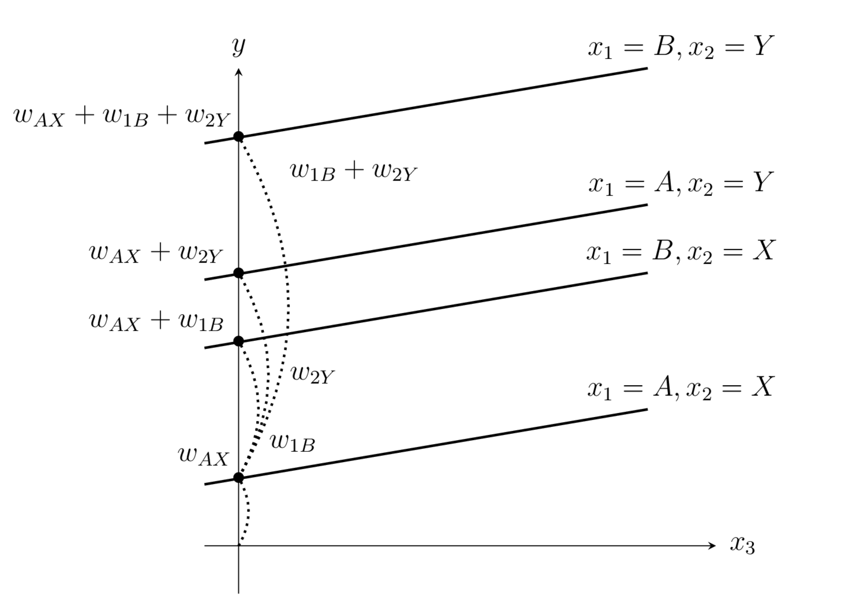
두 개 이상의 범주형 변수가 있는 경우에는 축소형 방식을 사용한다. 이 때 주의할 점은 모든 범주형 범수의 가중치는 기준값 상수항에 더해지는 상수항으로 취급된다. 예들 들어 \(x_1\)은 A, B 의 두가지 값을 가지고 \(x_2\)은 X, Y의 두가지 값을 가지고 값을 가지는 경우 상수항과 각 더미변수의 가중치의 의미는 다음과 같아진다.
\(w_{AX} \): 기준값 \(x_1=A, x_2=X\)인 경우의 상수항
\(w_{1,B}\): 기준값 \(x_1=B, x_2=X\)인 경우에 추가되는 상수항
\(w_{1,Y}\): 기준값 \(x_1=A, x_2=Y\)인 경우에 추가되는 상수항
\(w_{1,B} + w_{1,Y}\): 기준값 \(x_1=B, x_2=Y\)인 경우에 추가되는 상수항
%%tikz -p kotex,pgfplots -l arrows.meta,calc -s 2000,1200 -f png

\coordinate (leftbottom) at (-0.5,0);
\coordinate (righttop) at (12,9);
\fill[white,use as bounding box] (leftbottom) rectangle (righttop);
\draw[help lines, white] (leftbottom) grid (righttop);
\tikzset{
    >=stealth,font={\ttfamily\large}
}

\node (origin) at (3,1) {};

\draw[->] (3,0.3)--(3,8);
\node at (3,8.3) {$y$};
\draw[->] (2.5,1)--(10,1);
\node at (10.4,1) {$x_3$};

\draw[line width=1pt] (2.5,1.9)--(9,3);
\node at (9.5,3.3) {$x_1=A,x_2=X$};
\node(wAX) at (3,2) {};
\draw[fill] (wAX) circle (2pt);
\node at (2.5,2.3) {$w_{AX}$};

\draw[line width=1pt] (2.5,3.9)--(9,5);
\node at (9.5,5.3) {$x_1=B,x_2=X$};
\node(w1B) at (3,4) {};
\draw[fill] (w1B) circle (2pt);
\node at (1.8,4.3) {$w_{AX} + w_{1B}$};

\draw[line width=1pt] (2.5,4.9)--(9,6);
\node at (9.5,6.3) {$x_1=A,x_2=Y$};
\node(w2Y) at (3,5) {};
\draw[fill] (w2Y) circle (2pt);
\node at (1.8,5.3) {$w_{AX} + w_{2Y}$};

\draw[line width=1pt] (2.5,6.9)--(9,8);
\node at (9.5,8.3) {$x_1=B,x_2=Y$};
\node(wBY) at (3,7) {};
\draw[fill] (wBY) circle (2pt);
\node at (1.3,7.3) {$w_{AX} + w_{1B} + w_{2Y}$};

\draw[dotted, line width=1pt] (origin.center) edge[bend right] (wAX.center);
\draw[dotted, line width=1pt] (wAX.center) edge[bend right] (w1B.center);
\draw[dotted, line width=1pt] (wAX.center) edge[bend right] (w2Y.center);
\draw[dotted, line width=1pt] (wAX.center) edge[bend right] (wBY.center);

\node at (3.8,2.5) {$w_{1B}$};
\node at (4.1,3.5) {$w_{2Y}$};
\node at (4.7,6.5) {$w_{1B}+w_{2Y}$};
범주형 독립변수와 실수 독립변수의 상호작용#
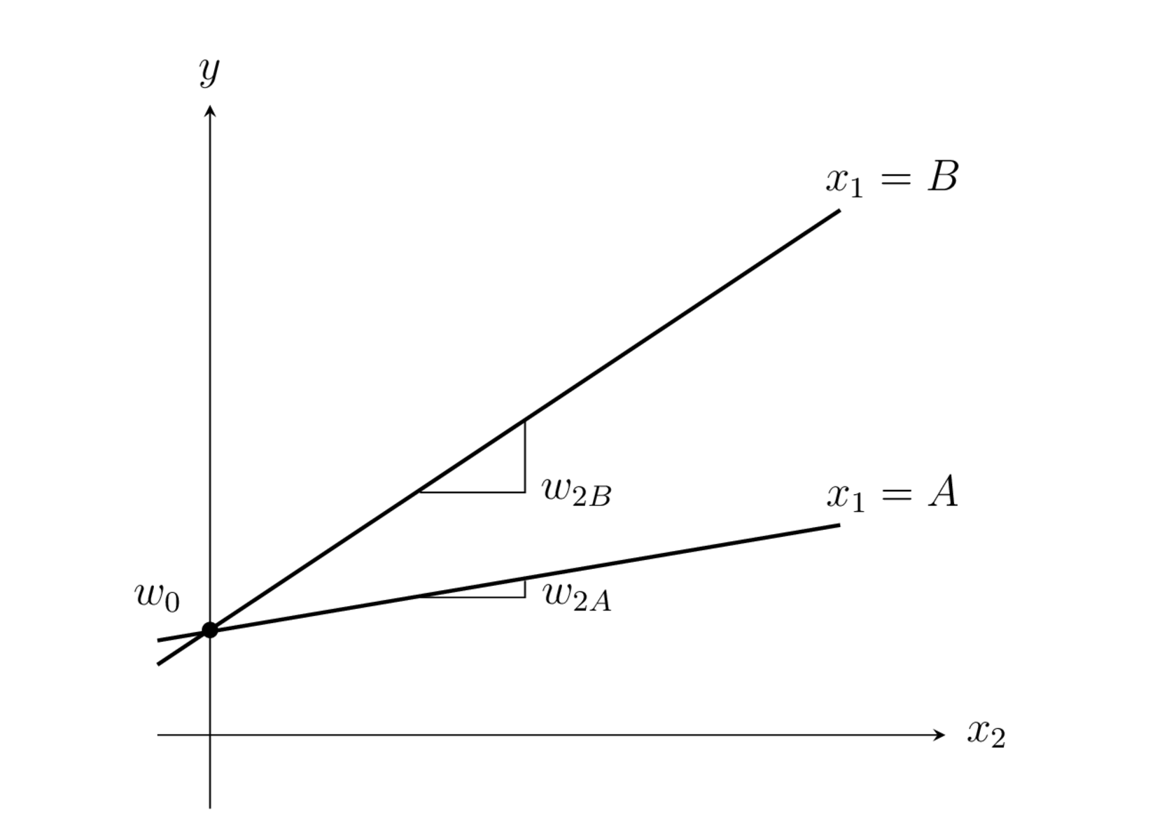
만약 범주형 변수의 값이 달라질 때 상수항만 달라지는 것이 아니라 다른 독립변수들이 미치는 영향도 달라지는 모형을 원한다면 상호작용(interaction)을 쓰면 된다. 예를 들어 범주형 독립변수 \(x_1\)과 실수 독립변수 \(x_2\)를 가지는 회귀모형에서 연속값 독립변수 \(x_2\)가 미치는 영향 즉 가중치가 범주형 독립변수 \(x_1\)의 값에 따라 달라진다면 범주형 독립변수를 더미변수 \(d_1\)으로 인코딩하고 연속값 독립변수 \(x_2\)는 \(d_1\)과의 상호작용 항 d_1:x_2 를 추가하여 사용한다.
이 때 모형은 다음과 같아진다.
\(x_1=A\)일 때는 \(d_A=1,d_B=0\)에서
\(x_1=B\)일 때는 \(d_A=0,d_B=1\)에서
이므로 \(x_1\) 범주값에 따라 \(x_2\)의 기울기가 달라지는 모형이 된다.
%%tikz -p kotex,pgfplots -l arrows.meta,calc -s 2000,1200 -f png

\coordinate (leftbottom) at (1,0);
\coordinate (righttop) at (12,8);
\fill[white,use as bounding box] (leftbottom) rectangle (righttop);
\draw[help lines, white] (leftbottom) grid (righttop);
\tikzset{
    >=stealth,font={\ttfamily\large}
}

\node (origin) at (3,1) {};

\draw[->] (3,0.3)--(3,7);
\node at (3,7.3) {$y$};
\draw[->] (2.5,1)--(10,1);
\node at (10.4,1) {$x_2$};

\draw[line width=1pt] (2.5,1.9)--(9,3);
\node at (9.5,3.3) {$x_1=A$};
\node(wAX) at (3,2) {};
\draw[fill] (wAX) circle (2pt);
\node at (2.5,2.3) {$w_{0}$};

\draw[line width=1pt] (2.5,1.67)--(9,6);
\node at (9.5,6.3) {$x_1=B$};

\draw (5,2.31) coordinate (w2A) -- ++(1,0) -- ++(0,0.16);
\node at ($(w2A)+(1.5,0)$) {$w_{2A}$};
\draw (5,3.31) coordinate (w2B) -- ++(1,0) -- ++(0,.7);
\node at ($(w2B)+(1.5,0)$) {$w_{2B}$};
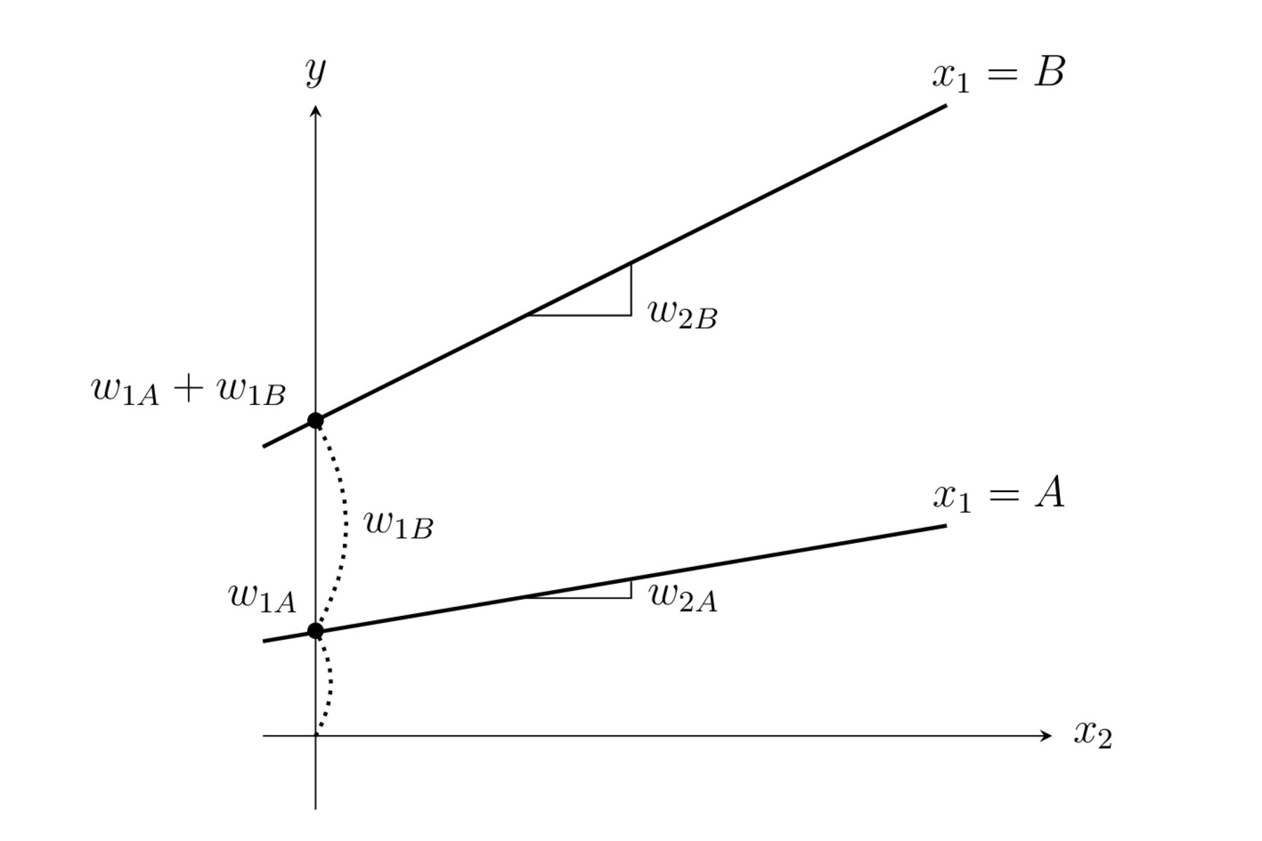
만약 범주형 독립변수도 종속변수에 영향을 미치고 범주형 독립변수와 실수 독립변수의 상호작용도 종속변수에 영향을 미친다면 모형은 다음과 같아진다.
\(x_1=A\)일 때는 \(d_A=1,d_B=0\)에서
\(x_1=B\)일 때는 \(d_A=0,d_B=1\)에서
이므로 \(x_1\) 범주값에 따라 상수항과 \(x_2\)의 기울기가 모두 달라지는 모형이 된다.
%%tikz -p kotex,pgfplots -l arrows.meta,calc -s 2000,1200 -f png

\coordinate (leftbottom) at (0,0);
\coordinate (righttop) at (12,8);
\fill[white,use as bounding box] (leftbottom) rectangle (righttop);
\draw[help lines, white] (leftbottom) grid (righttop);
\tikzset{
    >=stealth,font={\ttfamily\large}
}

\node (origin) at (3,1) {};

\draw[->] (3,0.3)--(3,7);
\node at (3,7.3) {$y$};
\draw[->] (2.5,1)--(10,1);
\node at (10.4,1) {$x_2$};

\draw[line width=1pt] (2.5,1.9)--(9,3);
\node at (9.5,3.3) {$x_1=A$};
\node(wAX) at (3,2) {};
\draw[fill] (wAX) circle (2pt);
\node at (2.5,2.3) {$w_{1A}$};

\draw[line width=1pt] (2.5,3.75)--(9,7);
\node at (9.5,7.3) {$x_1=B$};
\node(w1B) at (3,4) {};
\draw[fill] (w1B) circle (2pt);
\node at (1.8,4.3) {$w_{1A} + w_{1B}$};

\draw[dotted, line width=1pt] (origin.center) edge[bend right] (wAX.center);
\draw[dotted, line width=1pt] (wAX.center) edge[bend right] (w1B.center);

\node at (3.8,3) {$w_{1B}$};


\draw (5,2.31) coordinate (w2A) -- ++(1,0) -- ++(0,0.16);
\node at ($(w2A)+(1.5,0)$) {$w_{2A}$};
\draw (5,5) coordinate (w2B) -- ++(1,0) -- ++(0,.5);
\node at ($(w2B)+(1.5,0)$) {$w_{2B}$};